Lecture
When implementing simulation algorithms on digital machines, there are certain general patterns that we will discuss in this lecture.
The main problem in the compilation of algorithms on a machine with sequential processing of processes is that when modeling it is necessary to track many processes that occur in real time in parallel. In this regard, the simulation algorithms have their own characteristics:
At the moment, there are four basic principles for the regulation of events.
Let us consider with examples how each principle is implemented in modeling algorithms separately.
The principle is that the simulation algorithm simulates motion, that is, a change in the state of the system, at fixed points in time: t , t + Δ t , t + 2Δ t , t + 3Δ t , ...
For this, a time counter (clock) is started, which in each cycle increases its value t by the step size in time Δ t , starting from zero (the beginning of the simulation). Thus, changes in the system are monitored cycle by cycle at given times: t , t + Δ t , t + 2Δ t , t + 3Δ t , ...
This is the most universal of the considered principles, as it is applied to a very wide class of systems. It is also the simplest to implement, since the principle of Δ t coincides with a person’s understanding of time, as a sequential phenomenon flowing at a constant pace.
However, this is the most uneconomic principle, since the entire system is analyzed by a modeling algorithm on every clock cycle, even if there are no changes in it.
Another disadvantage is that the times of events are rounded to the value of Δ t , which leads to errors in determining the variables characterizing the system.
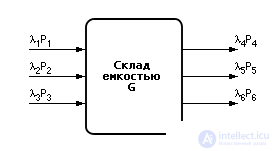
Consider an example. A warehouse of products with a maximum capacity G is simulated (see fig. 32.1).
| |
| Fig. 32.1. Scheme of the simulated production system (example) |
The warehouse accepts products from three suppliers (we denote the number of input flows of products 1, 2, 3) and issues them to three consumers (we denote the number of output flows of products 4, 5, 6). Let us take as the characteristic of each input the intensity of the i -th product flow ( λ i ). The intensity characterizes, on average, the distance between two points in time for arrivals (departures) of products to the warehouse. Let P i denote the size of the batch of products leaving or entering the warehouse. That is, these variables we determined when and how many products come or go to a particular entrance or exit of a warehouse ( block 1 - hereinafter see the blocks in Fig. 32.2).
Denote by variable Z the current number of items in stock. If the products arrive at the warehouse (flows 1, 2, 3), then Z is increased by P 1 , P 2 or P 3 . If items are withdrawn from stock (flows 4, 5, 6), then Z is reduced by P 4 , P 5 or P 6 . That is, Z plays the role of a counter for products that are in stock at a particular point in time t . The initial state of the warehouse at time t : = 0 will take Z : = Z 0 .
The algorithm will be constructed in such a way as to calculate the probabilities of events of occurrence of a deficit P d and overflow P p in stock.
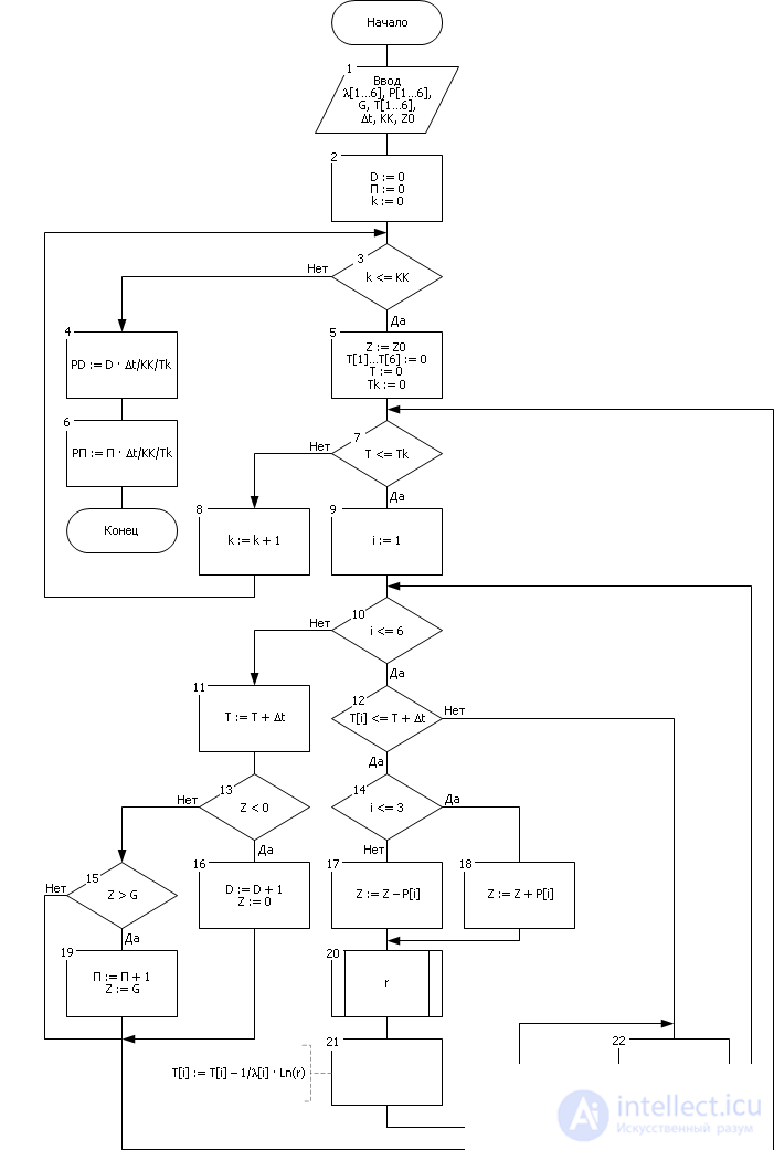
To accumulate reliable statistics, the experiment is repeated K K times. The number of experiments is monitored by the experiment counter k ( blocks 2, 3, 8 ). Each experiment lasts from 0 to T k point of time ( blocks 5, 7 ). The time counter t counts the time from 0 to T k with discreteness Δ t ( block 11 ).
In each experiment, it is calculated how many times in the warehouse as a result of input signals (the number of delivered and withdrawn items) a deficit situation occurs ( block 13 ). This is monitored by counter D , if a situation occurs in the warehouse Z <0 ( block 13 ), then there is a shortage of processing products and the counter increases its value by 1 ( block 16 ). If the deficit does not occur Z ≥ 0, then the counter does not change its value.
Since the total can be considered N : = T k / Δ t cycles, the probability of a deficit can be roughly estimated by the frequency of occurrence of these events as P d : = D / N or taking into account that the counter D accumulated during the KK experiments, P d : = D / N / KK . Finally, substituting N : P d : = D · Δ t / T k / K K ( blocks 4, 6 ). The calculation of the overflow probability of a warehouse is modeled in the same way (it is taken into account that overflow occurs when Z becomes greater than the capacity of warehouse G ) ( blocks 15, 19 ).
Note that since in stock, in reality, there can be no items less than zero, the Z value at the moment of detecting this fact should be returned to the nearest border, that is: Z : = 0 ( block 16 ). The same applies to the overflow situation ( Z : = G ) ( block 19 ).
The algorithm represents a failure cycle in time from 0 to T k with a step Δ t - the simulation is performed in time. In each cycle (at each time step), it is checked whether the generated T i event lies in the time interval [ T , T + Δ t ]: T ≤ T i < T + Δ t ( block 12 ). If an event occurs at a given moment, it is determined which i- th input signal predetermined this event ( blocks 22, 10 ), the situation is processed ( block 17 or 18 ) and the time of the next event is generated ( blocks 20, 21 ). The check on each clock cycle occurs on all possible input and output signals.
The block diagram of the algorithm is shown in Fig. 32.2.
| |
| Fig. 32.2. The block diagram of the algorithm implemented on the principle of Δt. Example - modeling of a production warehouse |
Let's call the state in which the system is usually the normal state. Such states of interest do not represent, although they occupy most of the time.
Special states are those at isolated points in time, in which the characteristics of the system change abruptly. To change the state of the system need a specific reason, for example, the arrival of the next input signal. It is clear that from the point of view of modeling, it is of interest to change the characteristics of the system, that is, the principle requires us to track the moments of transition of the system from one particular state to another.
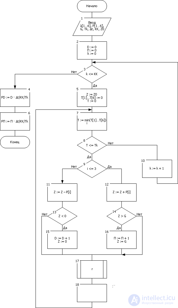
Compared with the previous case, we will not check the change in the state of the system at each moment in time. Among the future moments, we will select only those in which the products arrive or leave the warehouse closest to the current point in time ( block 7 - hereinafter see the blocks in Fig. 32.3). Having determined such a moment, we will immediately jump into it by changing the time counter value by the value (–Ln ( r ) / λ i ) ( block 18 ). Otherwise, the algorithm is similar to the previous one. We only note that the cycle of polling the input signals is eliminated, since block 7 clearly answers the question which of the i-th signals occurred.
All this significantly saves modeling time.
The block diagram of the algorithm is shown in Fig. 32.3.
| |
| Fig. 32.3. A block diagram of an algorithm implemented according to the principle of special states. Example - modeling of a production warehouse |
The principle is that each application is tracked from the moment it enters the system until it leaves the system. And only then the next application is considered.
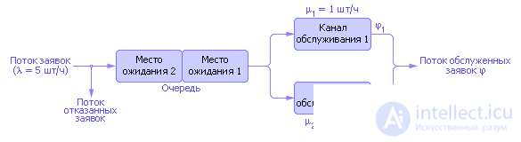
Consider the operation of the algorithm on the example of a two-channel queuing system with two places in a common queue with FIFO discipline and failures when the queue is full (see Fig. 32.4), see also Lecture 30.
| |
| Fig. 32.4. Queuing system diagram with two channels and limited queue |
Denote: λ - the intensity of the arrival of the application; μ i - the intensity of service applications.
We construct an algorithm that determines the probabilities of servicing requests and refusals of requests, as well as the system capacity.
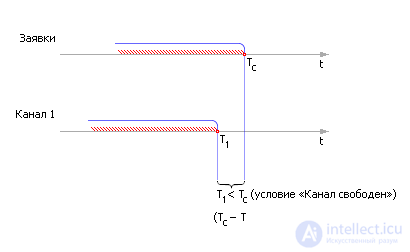
To understand the operation of the algorithm, imagine for clarity the parallel rulers — the time axes for each of the places where the application may be in the service process — as we did before (see Lecture 30).
We generate an application ( blocks 3, 4 - hereinafter see the blocks in Fig. 32.6). The random point in time when the application came into the system is equal to T with . The time between two random requests is simulated by the formula τ : = –1 / λ · Ln ( r ), which is added to T from the previous application T with : = T with –1 / λ · Ln ( r ). We take this fact into account in the counter of incoming applications N ( block 4 ).
We successively compare T with in order of priority ( blocks 5, 6, 7, 8 ) with release times T 1 of channel 1, channel 2 - T 2 , places in line 1 - T 3 , places in line 2 - T 4 . As soon as the fact is revealed that the place in the system is free (see Fig. 30.5): T with > T 1 , or T with > T 2 , or T with > T 3 , or T with > T 4 , so immediately translate the application to free space and simulate processing it at this place.
| |
| Fig. 32.5. The mechanism for determining the release of the channel (illustration) |
Suppose that a place is made in the first channel. Processing is that the idle time of this channel is calculated before the arrival of the request (for example, T with - T 1 ), and this time is added to the idle time counter ( block 15 ). The next time for changing the state of the channel is calculated - the variable T 1 is modified, which will tell us later when the channel is released again. The value of T 1 changes by the value τ : = –1 / μ 1 · Ln ( r ) - the service time counted from the beginning of the service T s . The counter of the served requests N about increases by unit.
Similarly, the processing takes place in the second channel, if the application gets exactly there ( block 14 ).
A feature of processing an application in a queue is that the first place in a queue is released when a place is released in one of the channels, of course, the application goes to where the space is released earlier ( blocks 5, 6 ). The second place in the queue is released simultaneously with the first, since the application in the queue moves to the first vacant seat ( block 12 ).
Next, the algorithm generates the following application in a loop ( blocks 3, 16 ). The simulation stops when each ruler is filled up to the time T k ( block 16 ). After this, the statistical results accumulated in the counters are processed ( block 17 ). The probability is estimated by the frequency of the occurrence of an event, which is calculated as the ratio of the number of events that have appeared to the number of possible such occurrences.
The block diagram of the algorithm is shown in Fig. 30.6.
| |
| Fig. 32.6. The flowchart of the algorithm implemented on the principle of sequential posting applications. Example - queuing system simulation |
And, of course, we must remember that the longer the simulation time, the more accurate the calculated result will be.
It makes sense to remind once again that it is necessary to observe the behavior of a statistical characteristic, which, for example, is P vol . Earlier (see Lecture 21, Lecture 34) we noted that the statistic changes with the observation time. As soon as the statistical value ceases to vary within the limits of the declared accuracy, that is, the curve enters the corridor assigned to it by precision, this indicates the sufficiency of the number of experiments.
Care must be taken to ensure that all the desired variables are included in the interval of the declared accuracy, only then can we stop the simulation and be confident in the result.
To increase the efficiency of the algorithm (reducing its time of operation), it is possible to discard the uncharacteristic part of the implementation - usually this is the initial part of the system’s work, “its exit to the mode”.
We also note that it does not matter whether we are dealing with a single long implementation or with a large number of short realizations (which, of course, cut out the “exit to mode” section), which together give a realization of the same length — the statistical result will be the same. This reasoning establishes the equality of averaging over an ensemble of realizations with averaging over time.
Note In practice, usually used combinations of all three methods.
As a rule, algorithms designed according to the first three principles are poorly upgraded. And the production situation often changes and requires appropriate models for finding rational decisions in the management process.
Thus, there was a need for modeling techniques that ensure the independence of the compilation of models of elements of a complex system from changes in the task or structure of production. Such an approach to modeling individual objects independently of each other allows you to collect arbitrarily complex systems without changing their components . The principle of object modeling provides modernization of complex systems, extending the life cycle of the ACS.
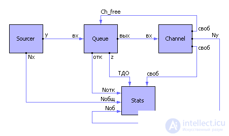
Example. The QS consists of the following elements existing by themselves: the source of applications, the queue, the channel (see Fig. 36.7). Let's model them separately.
| |
| Fig. 32.7. The implementation scheme of object-oriented modeling (for example, QS) |
1. Source of applications (Sourcer) generates a sequence of random events.
|
2. Channel service.
|
3. Queue.
|
4. Stats.
|
These models can be collected in any configuration without changing their content.

Comments
To leave a comment
System modeling
Terms: System modeling