Lecture
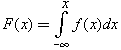
For the engineer, the law of probability distribution of a random variable X has a greater information content, as compared with such statistical characteristics as expectation, variance. Imagine that X takes random values from a certain range. For example, X is the diameter of the part being machined. The diameter may deviate from the planned ideal value under the influence of various factors that cannot be taken into account, so it is a random, poorly predictable value. But as a result of a long observation of the parts produced, it can be noted how many parts out of 1000 had a diameter of X 1 (we denote N X 1 ), how many parts had a diameter of X 2 (we denote N X 2 ) and so on. As a result, it is possible to construct a histogram of the particular diameters, postponing for X 1 the value of N X 1/1000, for X 2 the value of N X 2/1000 and so on. (Note, to be precise, N X 1 is the number of parts whose diameter is not just equal to X 1 , but is in the range from X 1 - Δ / 2 to X 1 + Δ / 2, where Δ = X 1 - X 2 ). It is important that the sum of all the frequencies will be equal to 1 (the total area of the histogram is unchanged). If X changes continuously, a lot of experiments have been carried out, then in the limit N -> ∞ the histogram turns into a graph of the probability distribution of a random variable. In fig. 24.1, and an example of a histogram of a discrete distribution is shown, and in fig. 24.1, b shows a variant of the continuous distribution of a random variable.
|
|
| Fig. 24.1. Comparison of discrete and continuous laws of random variable distribution |
In our example, the distribution law of the probability of a random variable shows how likely one or another value of the diameter of the parts produced is. The random variable is the diameter of the part.
In production and technology, often such distribution laws are given according to the condition of the problem. Our task now is to learn how to imitate the appearance of specific random events according to the probabilities of such a distribution.
Since the probability distribution laws of events can be of various forms, and not only equiprobable, it is necessary to be able to turn a uniform RNG into a random number generator with a given arbitrary distribution law. In fig. 21.3, this corresponds to the first two blocks of the statistical modeling method. To do this, the continuous law of probability distribution of an event is discretized, turned into a discrete one.
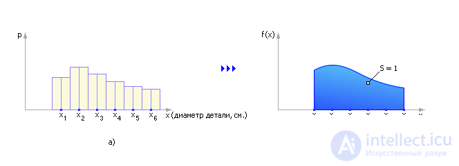
Denote: h i is the height of the i- th column, f ( x ) is the probability distribution (shows how likely some event x is ). The value of h i by the normalization operation must be converted into units of the probability of the occurrence of x values from the interval x i < x ≤ x i + 1 : P i = h i / ( h 1 + h 2 + ... + h i + ... + h n ).
The normalization operation provides the sum of the probabilities of all n events equal to 1:

In fig. 24.2 are shown graphically the transition from an arbitrary continuous distribution law to a discrete one (Fig. 24.2, a), the mapping of the obtained probabilities to the interval r pp [0; 1] and the generation of random events using a standard uniformly distributed RNG (Fig. 24.2, b).
|
|
| Fig. 24.2. Stepwise Approximation Method Illustration |
Note that within the interval x i < x ≤ x i + 1, the value of x is now indistinguishable, the same. The method coarsens the initial formulation of the problem, moving from a continuous law of distribution to discrete. Therefore, one should take into account the number of partitions of n from the conditions of accuracy of the representation.
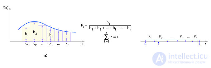
In fig. 24.3 the fragment of the algorithm realizing the described method is shown. The algorithm generates a random number uniformly distributed from 0 to 1. Then, comparing the boundaries of segments located on the interval from 0 to 1, representing the probabilities P of the occurrence of certain random variables X , determines in the loop which random event i as a result falls out.
|
|
| Fig. 24.3. Block diagram of the algorithm that implements step approximation method |
Note that within the interval x i < x ≤ x i + 1, the value of x is now indistinguishable, the same. The method coarsens the initial formulation of the problem, moving from a continuous law of distribution to discrete. Therefore, one should take into account the number of partitions of n from the conditions of accuracy of the representation.
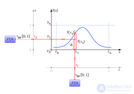
The method is used in the case when the function is specified analytically (as a formula). The graph of the function is entered in a rectangle (see. Fig. 24.4). On the Y axis serves a random evenly distributed number from the RNG. On the X axis serves a random evenly distributed number from the RNG. If the point at the intersection of these two coordinates lies below the probability density curve, then an X event has occurred, otherwise it does not.
The disadvantage of the method is that those points that turned out to be higher than the probability density distribution curve are discarded as unnecessary, and the time spent on their calculation turns out to be in vain. The method is applicable only for analytical probability density functions.
|
|
| Fig. 24.4. Illustration of the truncation method |
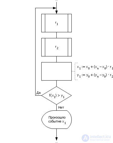
In fig. 24.5 shows the algorithm that implements the truncation method. The cycle generates two random numbers from the range from 0 to 1. The numbers are scaled to the X and Y scale and the point with the generated coordinates is checked under the graph of the given function Y = f ( X ). If a point is under the graph of the function, then event X occurred with probability Y , otherwise the point is discarded.
|
|
| Fig. 24.5. Block diagram of the algorithm that implements the truncation method |
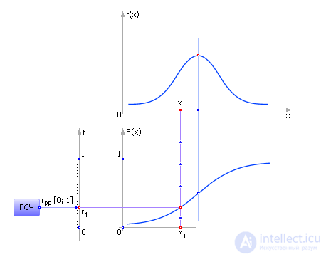
Suppose that we are given an integral probability distribution law F ( x ), where f ( x ) is a probability density function and
Then it is enough to play a random number evenly distributed in the interval from 0 to 1. Since the function F also changes in this interval, the random event x can be determined by taking the inverse function graphically or analytically: x = F –1 ( r ). Here r is the number generated by the reference RNG in the range from 0 to 1, x 1 is the random value generated as a result. Graphically, the essence of the method is shown in Fig. 24.6.
|
|
| Fig. 24.6. Illustration of the inverse function method for random generation x events whose values are distributed continuously. The picture shows graphs of probability density and integral probability density from x |
This method is especially convenient to use in the case when the integral law of probability distribution is given analytically and possibly analytically taking the inverse function of it, as shown in the following example.
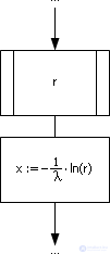
Example 1. Let us consider an exponential law of probability distribution of random events f ( x ) = λ · e - λ x . Then the integral law of probability density distribution has the form: F ( x ) = 1 - e - λ x .
Since r and F in this method are assumed to be similar and are located in the same interval, then replacing F with a random number r , we have: r = 1 - e - λ x .
Expressing the desired value of x from this expression (that is, reversing the function exp () ), we get: x = –1 / λ · ln (1 - r ).
Since in the static sense (1 - r ) and r are the same, x = –1 / λ · ln ( r ).
In fig. 24.7 shows a fragment of the algorithm that implements the inverse function method for the exponential law.
|
|
| Fig. 24.7. Fragment of flowchart, implementing the inverse function method for exponential law |

Comments
To leave a comment
System modeling
Terms: System modeling