Partial differential equations

Cases of the analytical description of systems with distributed parameters, partial differential equations are known from mathematics and physics. They are the equations of diffusion, heat and mass transfer, and others. Consider the options for their simulation on the computer.

Once again we recall that systems with distributed parameters are systems in which the value of some parameter under study changes not only in time but also in space (one-, two- or multidimensional), varying from point to point in space according to some law . An example of such a parameter is energy, substance concentration, field strength, and other physical quantities. The parameter under study can be considered unchanged only in an infinitely small region of space. Therefore, a system with distributed parameters is often represented as a system from a set of elements arranged in space, within which (at each point of an individual element taken) the described parameter is the same, but different for different elements. Elements of the system form a spatial structure.

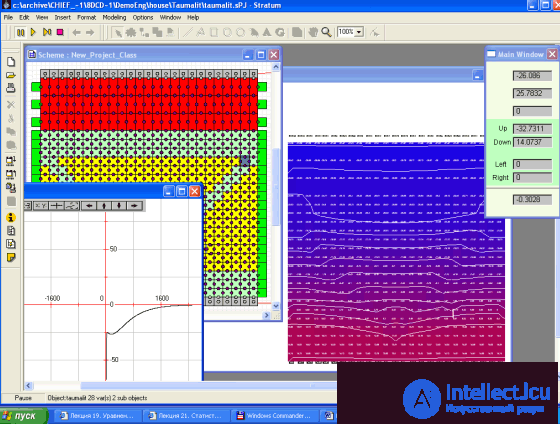
As an example, we give a project to study the thermal conductivity of the wall of a house. In fig. 19.1. The implementation of such a system in the Stratum-2000 environment is presented. The scheme is assembled from elements (images). Elements of a two-dimensional system mimic the bricks that make up the wall. Figure 19.1 visible bricks made of different materials (indicated by yellow, blue, red colors) and laid in a certain order, which, according to the author of the scheme, improves the insulation of the room. Gray and green elements at the edges of the wall set the boundary conditions, imitating the environment. The series shows for example how elements in such a system are related to each other. For connections, neighboring elements in the calculation process exchange information among themselves about temperature. Note that in this project, which has the form of a designer, the user of the scheme can change the parameters of the system elements, conditions, wall construction, installation procedure (topology), which is extremely difficult when solving a problem with analytical methods and requires the use of modeling methods.

Fig. 19.1. Two-dimensional system with distributed parameters to study the properties of thermal conductivity of the wall of the house

There are typical equations describing individual properties of systems with distributed parameters. Consider them.

Diffusion equation

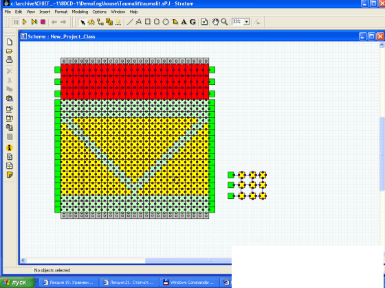
The diffusion equation describes the spread (spreading) with time over an extended body of a certain substance, for example, heat or concentration. In the one-dimensional case, the body is extended along the x axis.

In fig. 19.2 shows an example of the distribution along the x axis of such a parameter as temperature T. It is well known from ordinary experience that at each instant of time t, temperature T on different parts of the body x has different values, that is, varies depending on the area and time. That is, there must be a law according to which the value of this parameter T changes as a function of ( x , t ). For temperature, this law is most often given by the diffusion equation.

Fig. 19.2. An example of the use of the diffusion equation to the description of the process of heating an extended one-dimensional body

If the variable parameter (in the general case) is denoted as y , the time during which the parameter changes are tracked, denoted as t , and the axis along which the parameter changes occur as x , then the diffusion equation has the form:

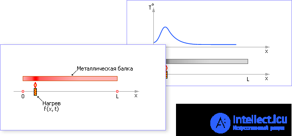
and is usually supplemented with conditions - the values ​​of the variable y at the edges and boundaries: on the left edge x = 0, on the right edge x = L , on the border - initial conditions ( t = 0):

y ( x , 0) = f ₁ ( x ),
y (0, t ) = f ₂ ( t ),
y ( L , t ) = f ₃ ( t ),
where f ₁ ( x ), f ₂ ( t ) and f ₃ ( t ) are given functions.

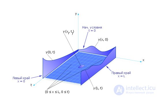
In fig. 19.3 shows a schematic view of the area for which the boundary and initial conditions are defined. The functions f ₁ ( x ), f ₂ ( t ), f ₃ ( t ) and the diffusion equation itself predetermine the behavior of the function y ( x , t ) within this region, whose full form should usually be determined. If the y- axis is additionally plotted (see Fig. 19.4), then the type of functions itself can be displayed visually in the figure. The figure clearly shows that in the corners of the circuit the values ​​of the specified functions must match.

Fig. 19.3. Scheme of the task of initial and boundary conditions for systems with distributed parameters in x, t axes (example)

Fig. 19.4. Scheme of the task of initial and boundary conditions for systems with distributed parameters in x, t, y axes (example)

The coefficient α has the meaning of the coefficient of thermal conductivity; f ( x , t ) has the meaning of a function describing the operation of sources and sinks of heat.

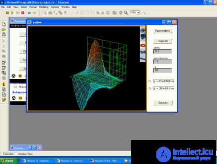
The quantity y , which describes the temperature distribution, is a function of two variables — the length of the body x and the time t : y ( x , t ). Graphically, the function is represented by a surface (see fig. 19.5) or a set of isolines (see fig. 19.6), the form of which is usually required to be determined.

Fig. 19.5. Calculation of heat distribution in a one-dimensional rod with time

Fig. 19.6. Heat distribution over the elements of a two-dimensional system (calculation static task presented in fig. 19.1). Visible in a separate window estimation of calculation accuracy depending on the number of iterations

If we replace the expressions of derivatives with their discrete analog, then in a difference form the equation will look like this:

or, expressing the unknown in terms of known quantities:

or

The result is a calculation formula that is implemented on a digital computer. Thanks to this formula, it is possible to calculate the value of the parameter y at any point ( x , t ).

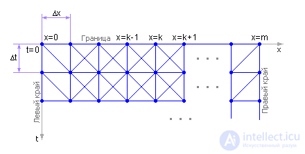
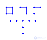
We call the value y ( x , t ) the calculation node. Then the calculation is schematically looks like a grid of nodes on the field, composed of body parts and time segments (see. Fig. 19.7). The formula for calculating a single node depends on the state of three nodes (left y ( x - Δ x , t - Δ t ), right y ( x + Δ x , t - Δ t ), proper y ( x , t - Δ t )) in the previous ( t - Δ t ) moment of time and resembles a triangular pattern. Before starting the calculation, the states of all nodes are known for t = 0. Applying the formula sequentially to all nodes for the next time point, it is possible to determine the temperature in all nodes of the next time layer ( t + Δ t ). In addition to the leftmost and rightmost nodes, their state cannot be calculated, but it is given by boundary conditions.

Fig. 19.7. The scheme for calculating a one-dimensional dynamic system with distributed finite difference parameters using an explicit template

If the procedure is repeated, moving from one point of the body x to another, and then from one time layer to another, then using this formula you can calculate the temperature value in any part of the body at any time. Thus, the calculation covers the entire field (L x T) (see fig. 19.7). The sequential determination of unknown values ​​in this case is possible, because the pattern has the form of an explicit expression — the only unknown in the formula is expressed in terms of previously calculated values.

Note that for large values ​​of the derivatives and large values ​​of the steps, the calculation may give incorrect solutions. Solutions may turn out to be inaccurate or even unstable (qualitatively incorrect) (see Lecture 10. “Numerical methods for integrating differential equations. Euler method”).

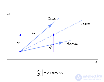
The stability condition for a triangular pattern when solving the diffusion equation: Δ x / Δ t > α (see Fig. 19.12 for more details).

When modeling, it is possible to use other difference formulas (templates) (see fig. 19.8). When choosing a template, it is necessary to take into account: an explicit template or not, which accuracy it provides and at what values ​​of steps it ensures stability of the calculation. So, for example, a pattern in the form of a rectangle is implicit: in one calculation formula two unknown quantities are contained at once. Therefore, when using such a template, it is necessary to solve a system of algebraic equations of size (L · T) .

Fig. 19.8. Typical Pattern Schemes to solve equations with distributed parameters

In practice, sustainability, and then accuracy, is achieved by obtaining solutions using different templates and different step values. If the values ​​of the desired variable, calculated with a step h and with a step h / 2, differ in nodes with the same indices by no more than 1–5%, then the calculated value is taken as an approximate solution of the problem. Otherwise, reduce the step twice, and the evaluation procedure is repeated. (For more, see the lecture “Can we calculate on a computer?”.)

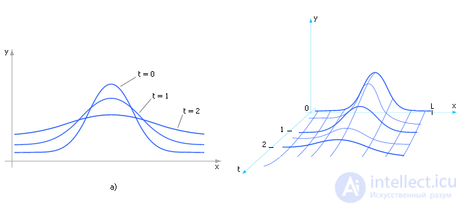
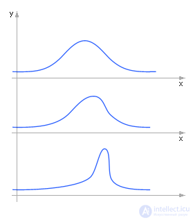
The properties of the diffusion equation are shown in Fig. 19.9 and consist in the fact that when a heterogeneity occurs in some part of the body, over time, heat due to heat transfer processes flows into neighboring areas. The temperatures of the neighboring areas are aligned, averaged. The rate of the process depends on the value of thermal conductivity.

Fig. 19.9. The characteristic form of the solution of the diffusion equation. The figure reflects the change the distribution of the parameter y along the x axis in time. a) - in two axes; b) - in three axes

If we accept the condition that the problem is stationary, that is, the processes take place so long that all transients have ended (the time derivative is 0), then the diffusion equation takes the following form (for the case of two-dimensional space - the x and z axes) without sources and sinks :

∂ ² y / ∂ x ² + ∂ ² y / ∂ z ² = 0.

In difference form, the equation has the form:

( Y _{i + 1, j} - 2 · Y _{i , j} + Y _{i - 1, j} ) / Δ x ² + ( Y _{i , j - 1} - 2 · Y _{i , j} + Y _{i , j + 1} ) / Δ z ² = 0.

If we take Δ x = Δ z , then the equation takes the form:

4 · Y _{i , j} - Y _{i + 1, j} - Y _{i - 1, j} - Y _{i , j - 1} - Y _{i , j + 1} = 0.

It is easy to understand that the template for calculating the equation is implicit and has the form of a cross (to calculate the temperature value at the grid node, you need to know the temperature of its neighbors on the left, right, top and bottom). If the wall of the house has dimensions of 2 meters by 2 meters, and the step Δ x = Δ z = 20 mm, then all to calculate the temperature regime of the wall will have to solve a system of 10,000 linear equations with 10,000 unknowns Y _{i , j} :

4 · Y _{i , j} - Y _{i + 1, j} - Y _{i - 1, j} - Y _{i , j - 1} - Y _{i , j + 1} = 0, for i = 1 ÷ 100 and j = 1 ÷ 100,

to which 400 pieces of boundary conditions should be attached:
Y _{0, j} = f ₁ ( j );
Y _{101, j} = f ₂ ( j );
Y _{i , 0} = f ₃ ( i );
Y _{i , 101} = f ₄ ( i ).

The type of solution of the equation is shown in fig. 19.6.

Heat and mass transfer equation

In a number of physical processes, a mass of matter or energy moves inside an imaginary system, moving from one part of it to another. Such processes are described by the equation of heat and mass transfer. For the one-dimensional case, this equation has the following form: ∂ ρ / ∂ t + ∂ q / ∂ x = B , where ρ ( x , t ) is the density of the substance or energy; q ( x , t ) is the flow of matter or energy; B ( x , t ) is a function of sources and sinks. ρ ( x , t ), q ( x , t ), B ( x , t ) are the distribution functions of the corresponding variables in the space x and time t .

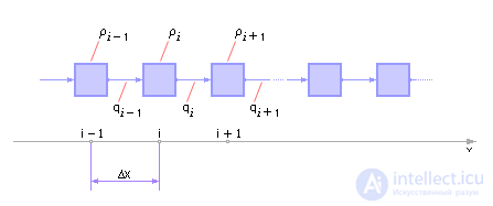
We divide the flow along the x axis into unit cells that interact with each other. Each cell is characterized by the density ρ of the substance in it and the flow of substance q through its borders (left and right). We number the cells by index i . A cell is usually called an elementary volume.

Fig. 19.10. Scheme of the heat equation (example)

In the difference form (after the substitution of expressions for the numerical calculation of derivatives), the heat equation will have the form:

The equation and the corresponding diagram in fig. 19.10 shows how much substance will be added in the elementary volume ∂ ρ / ∂ t in the time Δ t , if q ( x ) · Δ t particles of the substance flow through the left border of this area x during this time, and if through the right border of this area ( x + Δ x ) at the same time flows q · ( x + Δ x ) · Δ t particles of a substance, and there is a source or sink of a substance b in the area .

Depending on the problem being solved, the equation can be supplemented. The function b ( x , t ) is usually specified. If it is necessary to determine the law of motion of the substance q ( x , t ) to ensure the user-specified distribution of the substance along the x axis with time ρ ( x , t ), then one equation is sufficient for such a calculation.

If the law of motion of the substance q ( x , t ) is specified and it is required to determine where, as a result of this movement, when and how much substance is ρ ( x , t ), then one equation is also sufficient.

But it is often required to determine simultaneously both ρ ( x , t ) and q ( x , t ) under given initial conditions, that is, the question is how fast q ( x , t ) and how much ρ ( x , t ) of the substance will be in certain points x . Then a single equation for calculating two unknowns is not enough. And the basic equation should be supplemented with auxiliary expressions indicating how ρ ( x , t ), q ( x , t ) are related to each other. Such an expression should indicate how fast a substance moves, if its quantity is given. In production and technology, we call this expression a regulator: how is the number of parts ρ stored in area x related to the desired processing speed of such parts q .

Depending on the substance we are dealing with, there may be various expressions of an additional connection (an additional equation) between the flow q and the density ρ . For example, for a fluid, where all particles move simultaneously : q = ρ · v , where v is the velocity of movement of particles in the flow. Or a more complex equation of motion, which relates the flow velocity v ( x , t ) to the cause of this motion, the force F :

∂ v / ∂ t + v · ∂ v / ∂ x = F / ρ .

In turn, the force F can be caused to the action by the pressure drop P : F = ∂ P / ∂ x .

It is easy to see in this equation as its basis the Newton's second law, which relates the acceleration ∂ v / ∂ t and the force F through the mass ρ . The additional term v · ∂ v / ∂ x appears as long as during the movement there appears an inflow of substance through the boundaries x and ( x + Δ x ) of the elementary segment, which carries the impulse v · ∂ v / ∂ x · ρ .

In the difference form with q = ρ · v, the transfer equation will be:

The equation is calculated similarly to the diffusion equation.

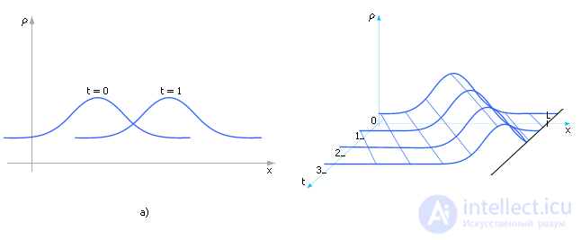
The properties of the transport equation consist in moving the inhomogeneities in the flow with time along the spatial axis. Movement speed is associated with v or q values. Figure 19.11 shows a view of one of the possible solutions to the heat and mass transfer equation. It is seen that the density distribution (inhomogeneity) can move along the axis with time.

Fig. 19.11. Properties of the equation of heat and mass transfer. a) - in two axes; b) - in three axes

Special attention when calculating an equation should be paid to its stability. Stability is associated with the type of the selected differential template and its parameters: t increments, x increments, and the speed (flow) of mass movement (see. Fig. 19.12). The greater the step, the greater the risk of obtaining unstable (qualitatively wrong) solutions. But the smaller the steps, the slower the computer calculation of the entire field, as the amount of calculations increases significantly.

Fig. 19.12. The ratio of the calculation parameters for a sustainable solution

In real systems, there are usually both diffusion properties and properties of the transport equation, motion. Therefore, the effects of transport and diffusion are mixed, and the paintings as a result of the calculation are quite complex, depending on the boundary and initial conditions and the ratio of the coefficients of the equations, as shown, for example, in Fig. 19.13.

Fig. 19.13. Type of possible solutions to the equation heat and mass transfer with diffusion elements. The figure shows the manifestation several properties simultaneously

Distributed systems include production systems (see Lecture 31. “Modeling of production processes and systems”).

One of the most difficult tasks considered in the class of systems with distributed parameters is the weather forecast. This takes into account temperature, pressure, wind speed, humidity, air density, terrain. All these quantities are a function of three spatial coordinates and time. 10 ⁶ initial data, not counting photographs, are subjected to analysis at weather forecasting centers daily. The calculation is made twice a day: at 00 o'clock and at 12 o'clock GMT. The exchange of measurement information between meteorological stations of different countries takes place within the framework of the World Meteorological Society, which includes the Russian Federation. On average, to calculate a single forecast, information from 4,000 surface sources (including 800 sea sources) and 650 air sources is taken into account. A network of measuring instruments covers the globe unevenly and this complicates calculations.

It is not difficult to estimate the average grid step. When the Earth’s radius is R = 6,400 km, the area of ​​the Northern Hemisphere is: S = 260,000,000 km ² . Thus, S / 650 = 400 000 km ² or a square with a side equal to the distance from Moscow to St. Petersburg falls on one aerostation. A square with a side of 300 km falls on one ground station. Such a step of the calculation grid leads to enormous difficulties in the struggle for the stability of the calculation.

Свои проблемы вносит и недостаточная точность исходных данных, поступающая от источников — погрешность измерений на море составляет обычно 10%, на суше — 15%.

При расчетах прогноза погоды кроме описанных уравнений дополнительно учитывают законы сохранения (массы, импульса, энергии), свойства вещества (Клаузиса-Клапейрона, Ван-дер Ваальса, фазовых переходов, поглощения солнечной энергии, излучения и другие). Учитывают также силы тяжести, вязкости, Кориолиса и другие. Расчет погоды ведут обычно на сверхмощных компьютерах типа Cray (см. видео Cray).