Lecture
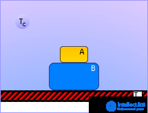
Perform the construction of a model of a dynamic system in the form of differential equations and its calculation by the Euler method using an example. Example. Let the system of two material bodies A and B with different thermal properties be investigated (see fig. 11.1). The system is in contact with a support with a temperature T p and placed in an external environment with a temperature T c . Interested in the process of changing the temperature of bodies.
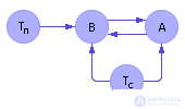
As can be seen, in the course of life in the system, four indicators change (may change): the temperatures of bodies A , B , T с , T p . This means that we are dealing with four time-dependent variables (since variables change their values with time). We introduce these variables: X 1 ( t ), X 2 ( t ), X 3 ( t ), X 4 ( t ). To build a mathematical model of this system, we reflect the heat transfer process in the form of a dependency graph (Fig. 11.2).
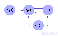
If we mean the variables X 1 ( t ), X 2 ( t ), X 3 ( t ), X 4 ( t ), then the graph will look like it is shown in Fig. 11.3.
The arrow from A to B denotes the change in temperature X 2 ( t ) of object B under the influence of object A. It is clear that a row of arrows (for example, from B to T c , from A to T p , etc.) is absent, that is, there is no effect of some parameters on others: body B is not able to heat the open atmosphere significantly, and body A - massive and potentially endless support. Strictly speaking, there is such an influence, but it is so insignificant that it is reasonable to neglect it. Since there are four variables, we need at least four laws describing their change. In general terms, considering which variables each indicator depends on, we get:
The arrows in the corresponding circle indicate the number of influencing parameters, and where they come from determines the specific names of the variables. For the environment, the law has the form: X 3 ( t ) = const, that is, the atmosphere temperature T с does not depend on the other components of this system and, accordingly, does not change. For a support, the law has the form: X 4 ( t ) = const, that is, the support temperature T n does not depend on the other components of this system and, accordingly, does not change. The system of laws in the first approximation is formed. It remains to determine their specific form: to reveal what the values of the expressions f 1 and f 2 are . Since we are dealing with a system that depends on its past behavior at each subsequent step, we used differential equations to describe it . The basic dynamic law for describing the change of a variable (the equation of motion) is: d X ( t ) / d t = w ( x ( t ), y ( t ), z ( t ), ...). The physical meaning of the recording is as follows. The derivative on the left side of the equation, by definition, shows how much X changes with a change in time t . In engineering, such a change is called speed, pace, trend. So, to write the law of variable change in differential equations, you must specify the rate of change of variables. First consider the first equation: d X 1 ( t ) / d t = f 1 ( X 1 ( t ), X 2 ( t ), X 3 ( t )). The appearance of X 1 on the right side means that the rate of temperature change depends on its own state of the body. What is f 1 ? Is a function that binds the variables X 1 , X 2 , X 3 to each other. That is, the variables are connected to each other by operation signs. Take a look at the graph in fig. 11.3. What pairs of variables interact? The arrows connect X 1 ( t ) with X 2 ( t ), X 1 ( t ) with X 3 ( t ), that is, there are two processes that affect speed. We consider the heat transfer processes of bodies. It is known that the two processes of heat transfer are independent, that is, they do not control each other. This means that the results of the two processes can be added, they seem to overlap each other. Indeed, the heat transferred from one body is added to the heat transferred from the other. Thus, we have: d X 1 ( t ) / d t = g 1 ( X 1 ( t ), X 2 ( t )) + g 2 ( X 1 ( t ), X 3 ( t )). We reveal the structure of the remaining expressions g 1 and g 2 . It is very convenient that g 1 does not depend on g 2 in any way and can be considered separately. This separation is possible because the processes g 1 and g 2 are independent. Process g 1 goes on regardless of whether or not process g 2 goes on . Process independence and linearity (additivity) of expressions are related concepts. So: since the processes g 1 and g 2 are independent, we forget for some time g 2 . What mark should be placed between X 1 ( t ) and X 2 ( t ) in the expression g 1 ? Possible options: X 1 ( t ) + X 2 ( t ); and further more complex, for example, X 1 2 ( t ) · cos ( X 2 ( t )) / exp ( X 1 ( t )). The researcher will start with the most simple expressions - nature is simple. And only if the simplest expressions do not satisfy the researcher, he proceeds to more complex versions of the description. What was just said above was elevated in system engineering to the rank of the principle: “do not introduce entities without need” (Occam's principle). So, let: d X 1 ( t ) / d t = X 1 ( t ) + X 2 ( t ). What are the quality options for this physical system?
Now let d x 1 ( t ) / dt = X 2 ( t ) - X 1 ( t ). What are the quality options for this physical system?
There are no other options for the existence of the system, and consideration ends. Having forgotten for some time about g 1 , it is also possible to consider g 2 , which is proposed to be done by the reader independently. In the end, we get: d X 1 ( t ) / d t = ( X 2 ( t ) - X 1 ( t )) + ( X 3 ( t ) - X 1 ( t )). Further. Since, firstly, for different materials the temperature difference affects the rate of change in body temperature in a different way and, secondly, the speed of the two processes (for two different pairs of materials) can be different, then we correct the model using the coefficient of thermal conductivity, which plays the role of the amplifier (attenuator) processes. This is the coefficient of influence of communication on the object. When K = 0, there is no influence, communication is disabled. At K = 0.0001, the effect is weak. With K = 1000, the effect of communication is enormous. It is clear that the coefficient is in the process expression: K ? ( X 2 ( t ) - X 1 ( t )), where « ? "Means the sign of some operation, namely, the multiplication operation. This operation gives the dependence of one member on the other (in our case, K on X 2 ( t ) - X 1 ( t )). When K = 0, whatever value the expression X 2 ( t ) - X 1 ( t ) takes , the result K · ( X 2 ( t ) - X 1 ( t )) gives 0. At K = 0.1, the value of the expression is forcibly weakened 10 times. The same is true of the expression X 2 ( t ) - X 1 ( t ) - this is natural, because the general expression K · ( X 2 ( t ) - X 1 ( t )) is symmetrical. This means that the multiplicative connection models the property of nonlinearity and interdependence of processes (one can negate the action of the other). Addition does not possess such a property. As a result, the model has the form: d X 1 ( t ) / d t = K 21 · ( X 2 ( t ) - X 1 ( t )) + K 31 · ( X 3 ( t ) - X 1 ( t )). At the end, check the dimensions of the equation; the dimension of the left side must coincide with the dimension of the right. We only recall that the derivative has the dimension of the index X divided by the unit of time. Now we are able to synthesize similarly the second equation (we recommend checking the correctness of this equation on our own): d X 2 ( t ) / d t = K 12 · ( X 1 ( t ) - X 2 ( t )) + K 32 · ( X 3 ( t ) - X 2 ( t )) + K 42 · ( X 4 ( t ) - X 2 ( t )). The equation for changing the temperature of the atmosphere: d X 3 ( t ) / d t = 0. That is, X 3 = const ( X 3 does not change). The equation for the temperature of the support: d X 4 ( t ) / d t = 0. That is, X 4 = const ( X 4 does not change). The entire system of equations in the collection has the form: For physical reasons, it is clear: how much heat flows from A to B , as much heat flows to B from A , that is, K 21 = K 12 . It remains to add specific values of thermal conductivity coefficients ( K 12 = K 21 , K 31 , K 32 , K 42 ) and the initial state of the system to the record of the general model: X 1 (0) = a , where a , b , c , d are numbers indicating the temperature of the corresponding object at time t = 0. |
|
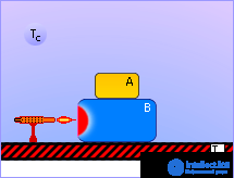
Important note. The work done above to confirm the hypotheses contained in the model of this example, of course, does not prove the absolute correctness of the adopted model. Checks can be continued. If at the next test the hypothesis is rejected, then the model should be clarified again . One of the additional checks may be, for example, checking for openness of the system. Perform this check. Note that above we got an open system , that is, one whose total heat is not constant, but may change. This is evident from the asymmetry of the arrows on the graph. Let us check this fact mathematically, formally, for which we add the left sides of all equations and, separately, the right sides. On the left we have the following: d X 1 ( t ) / d t + d X 2 ( t ) / d t + d X 3 ( t ) / d t + d X 4 ( t ) / d t or d ( X 1 ( t ) + X 2 ( t ) + X 3 ( t ) + X 4 ( t )) / d t or d X systems ( t ) / d t . On the right side we have the following: K 21 · ( X 2 ( t ) - X 1 ( t )) + K 31 · ( X 3 ( t ) - X 1 ( t )) + K 12 · ( X 1 ( t ) - X 2 ( t )) + K 32 · ( X 3 ( t ) - X 2 ( t )) + K 42 · ( X 4 ( t ) - X 2 ( t )) or (given that K 21 = K 12 ) K 31 · ( X 3 ( t ) - X 1 ( t )) + K 32 · ( X 3 ( t ) - X 2 ( t )) + K 42 · ( X 4 ( t ) - X 2 ( t )) . And finally, together: d X of the system ( t ) / d t = K 31 · ( X 3 ( t ) - X 1 ( t )) + K 32 · ( X 3 ( t ) - X 2 ( t )) + K 42 · ( X 4 ( t ) - X 2 ( t )), which means that the left side is clearly non-zero and there is a leak or heat influx into the system from the outside. In the case of a closed system, the equations would be: When added, this gives: d X of the system ( t ) / d t = 0 is the equation of a closed system into which nothing flows from outside and from which nothing flows. Although changes occur within the system (redistribution of heat), the total temperature of the system is unchanged. Neither the first model (open system model) nor the second model (closed system model) are “bad”. Simply achieved various goals, given the different views of the researcher about the processes of the system as a whole. The dynamic system , which we considered above, is a general case. It is very important that you can always get a static system out of it , for which you need to demand: X i ( t + Δ t ) = X i ( t ), with the result that we have: d X i ( t ) / d t = 0. In other words, the entry X i ( t + Δ t ) = X i ( t ) means that the past is equal to the present, that is, the state of the system does not change. Then from the equations remains: These are static equations. After building the base system, the researcher may introduce additional structural elements into the system of bodies. Add, for example, a heater (see fig. 11.4).
The graph will change, since an additional object - a heater will act on the body B. Denote its temperature by the variable X 5 ( t ) (see fig. 11.5).
Changes in the record will apply only to the second equation describing the change in the variable X 2 over time. In addition, we need the heater equation, since an additional variable X 5 ( t ) (the top of the graph) has appeared in the system and the law of its change must be determined. When writing the equation, it is necessary to distinguish whether the heat source is weak or strong. We first consider the hypothesis of a weak source. Pay attention: if the heater warms more strongly than body B , then, of course, body B heats up from the heater, but if the heater at some moment turns out to be colder than body B , then body B itself gives off heat to the heater, strange as it may seem nor seemed to. Since such a source of energy can not only heat up other bodies, but also heat itself from them, it is called weak. That is, the services of such an energy source can be waived, since it is in an equal position with other bodies, can influence them and may experience their influence. Other bodies cannot influence a strong source, and it itself - can influence them, BINDING THEM TO I WILL WILL OF CERTAINLY. It is clear that in the equation for body B there will appear an additional term similar to the previously considered ones: d X 2 ( t ) / d t = K 12 · ( X 1 ( t ) - X 2 ( t )) + K 32 · ( X 3 ( t ) - X 2 ( t )) + K 42 · ( X 4 ( t ) - X 2 ( t )) + K 52 · ( X 5 ( t ) - X 2 ( t )). The equation of the heater can be written as: d X 5 ( t ) / d t = ( K · U ( t ) - X 5 ( t )) / L + K 25 · ( X 2 ( t ) - X 5 ( t )), where U ( t ) is the supply voltage of the source. The initial conditions X 5 (0) and the source function U ( t ) must be specified: X 5 (0) = h , The equation relates the cause (voltage of the power supply) and the effect (temperature of the heater). The properties of this element are such that when entering the operating mode, the heater maintains a constant temperature. When the heater is turned on, the working temperature is set over time, gradually increasing, when the source is turned off, the heater gradually cools down. It is obvious that the process of heating and cooling the heater is inertial. In fact, to describe these properties of the heater, it suffices to write down the aperiodic law ( which we discussed earlier in lecture 04) of the change in its temperature X 5 ( t ) with respect to the input U ( t ), which we did. The equation takes into account the gain K between the input U ( t ) and the output X 5 ( t ), the inertia of the heating process L and the heat transfer coefficient K 25 between the bodies X 2 ( t ) and X 5 ( t ). Now consider the hypothesis of a strong heater. Это случай, когда нагреватель устроен таким образом, что излученная им энергия не может отразиться телом B , или если энергия от тела B не может попасть к нагревателю, или если тело B не может «отказаться» от услуг нагревателя (см.рис. 11.6).
In fig. 11.7 изображен граф зависимостей для данного случая.
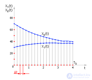
Обратите внимание: неважно, нагрет ли нагреватель сильнее тела B или нет — тело B будет получать от него энергию в любом случае, причем, в том объеме, в каком эту энергию будет выделять нагреватель. В уравнении тела B появится дополнительное слагаемое: d X 2 ( t )/d t = K 12 · ( X 1 ( t ) – X 2 ( t )) + K 32 · ( X 3 ( t ) – X 2 ( t )) + K 42 · ( X 4 ( t ) – X 2 ( t )) + K 52 · X 5 ( t ). Уравнение нагревателя может быть записано так: d X 5 ( t )/d t = f ( t ). Начальные условия X 5 (0) и функция работы источника f ( t ) должны быть заданы: X 5 (0) = h . Но вернемся к расчету движения во времени динамической системы, для которой есть все необходимые данные, есть начальное состояние ( X i (0) = const). Можно по формулам (с использованием метода Эйлера, см. лекцию 10) вычислить скорость ее изменения и новое состояние: новое состояние := старое состояние + скорость · отрезок времени . Формально эта запись выглядит так: d x ( t )/d t = f ( x ( t )) или (в дискретной форме) [ x ( t + Δ t ) – x ( t )]/Δ t = f ( x ( t )) и, окончательно, x ( t + Δ t ) = x ( t ) + f ( x ( t )) · Δ t . Зная новое состояние и считая его уже достигнутым, то есть старым состоянием , используем ту же формулу (подставляя, конечно, в нее уже новые значения). И так продолжаем, прибавляя все новый отрезок времени, двигаясь во времени. Итак, мы перешли к вопросу о методе расчета дифференциальных моделей. Методом решения дифференциальных уравнений, в общем случае, является интегрирование их по независимой переменной времени t . Простейшим методом численного интегрирования дифференциальных уравнений является метод Эйлера (см. лекцию 10). Обратите внимание. При вычислении по методу Эйлера необходимо вычислять значения всех параметров системы параллельно , так как производная в каждый момент времени отдельного параметра зависит как от значения самого параметра в данный момент времени, так и от значения другого параметра в этот момент времени. Рассмотрим практически применение метода Эйлера для расчета процесса изменения температур тел системы. Зададим значения коэффициентов модели: K 12 = K 21 = 0.2, K 31 = 0.1, K 32 = 0.05, K 42 = 0.1. Зададим начальные условия системы (в момент времени t = 0): X 1 (0) = 30° C, X 2 (0) = 70° C, X 3 (0) = 22° C, X 4 (0) = 15° C. Выбираем шаг моделирования Δ t равный, например, 0.2 с. Примем конечное значение времени моделирования за T k = 4 с. Подставим значения коэффициентов: и приступаем к моделированию. Процесс моделирования и численные значения отражены в табл. 11.1.
Во времени поведение системы будет выглядеть так, как показано на рис. 11.8.
Заметим, что на рис. 11.8 показана не вся траектория, а только ее часть. Рассчитайте всю траекторию, подумайте и ответьте на следующие вопросы:
В зависимости от реализации «машины», на которой автоматически будет имитироваться процесс, запись может выглядеть по-разному. Формальная математическая записьПриведем ниже вариант формальной математической записи для случая открытой системы тел со слабым нагревателем.
При реализации на математической машине среды Stratum эта запись будет дополнена элементами (функциями) ввода и вывода информации и командами управления (например, «стоп»), а часть элементов будет спрятана (например, при задании начальных условий). Иногда (когда это удобно) начальные условия могут быть помещены внутрь уравнений. Для этого в следующей записи мы воспользуемся дельта-функцией Дирака (см. лекцию 31).
Напомним, что osc2d( T , X 1 ) — функция, рисующая на экране точку с координатами T и X 1 для каждого момента времени. Выше данная функция приведена условно: в действительности надо использовать несколько функций для настройки окон, масштаба изображения, цвета, толщины, стиля линии и тому подобного. Подробно реализацию двухмерного осциллографа в среде «Stratum-2000» вы можете посмотреть в тексте имиджа OSCSpace2D. Приведенный выше вариант формальной математической записи подразумевает, что весь код заключен в рамках одного элемента (имиджа, если использовать термины среды «Stratum-2000»). Будет гораздо более наглядно, если распределить код по отдельным элементам, связав их между собой связями (см. рис. 11.9) — в этом случае структура проекта останется обозримой; кроме того, если потребуется изменить что-то в одном из блоков, то такой подход позволит не менять код в остальных блоках. Еще один плюс такого подхода — отдельные «кирпичики» схемы могут быть применены неоднократно в готовом виде в виде копии имиджа.
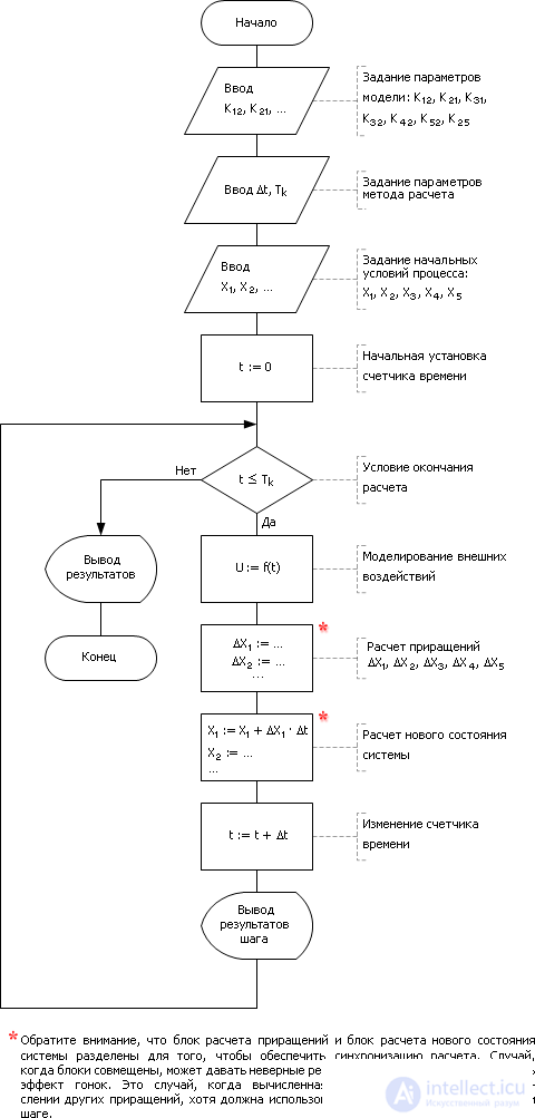
Алгоритмическая реализацияВ случае реализации на алгоритмической машине следует воспользоваться алфавитом алгоритмов: блоками начала и конца алгоритма, ввода-вывода информации, задания начальных условий, вычислительными блоками, блоками условия, конструкциями цикла. In fig. 11.10представлена блок-схема алгоритма, имитирующего теплообмен между телами.
Заметьте, что для реализации нам понадобились следующие инструменты:
В теле цикла присутствуют:
In one way or another, the above blocks are necessarily present in each algorithm of this type. |


Comments
To leave a comment
System modeling
Terms: System modeling