Lecture
The Euler method for calculating differential equations has a small calculation accuracy. As was shown earlier (see Lecture 10. Numerical methods for integrating differential equations. Euler's method), the accuracy of the calculation depends linearly on the step size, the dependence of the accuracy on the step is of the first degree. That is, to increase accuracy by 10 times, it is necessary to reduce the step by 10 times. In practice, they are interested in more advanced methods. The question is: is it possible to increase the accuracy by an order of magnitude, but at the same time save on the number of calculations? Yes, there are such methods. The modified Euler method has second-order accuracy. In the Euler method, the derivative is taken at the beginning of a step and it is predicted that the system will move to the end of the step, assuming that the derivative is constant during the step. That is, during the whole step, the derivative is considered to be what it was at the very beginning of the step. This is the main source of inaccuracy.
An improvement in the method is that the derivative is not taken at the beginning of the step, but as an intermediate or average in different parts of the same step. In different variants of the method, several derivatives are calculated in different parts of the step and averaged. Of course, in this case the number of calculations increases, but not by a dozen times, but the accuracy increases by an order of magnitude, this is the gain.
Let, as before (see Lecture 10. Numerical methods for integrating differential equations. Euler's method), it is required to solve the equation y ' = f ( x , y , t ). The idea of the refined Euler method is that the derivative is calculated not at the i -th point, but between two adjacent points: i and i + 1. This procedure consists of the following steps:
This method has an accuracy of Ο 2 ( h ), that is, an order of magnitude higher than the Euler method, with an increase in the number of calculations by a factor of 2.
In fig. Figure 14.1 shows what the error ε will be (the difference between the real and the calculated theoretical value) if the step is taken from the value of the derivative calculated at point i , as is done in the Euler method. This error can be quite large!
|
|
| Fig. 14.1. The movement of the real and accounting system according to the Euler method and the discrepancy between them (error) |
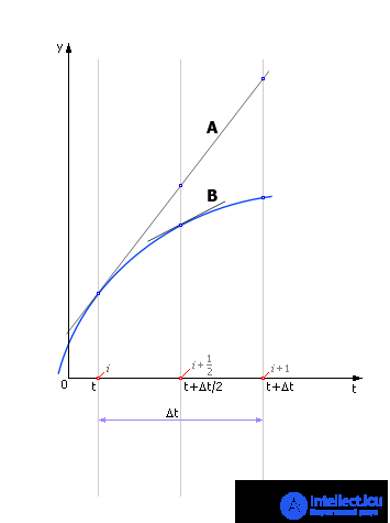
In fig. 14.2 it is shown how, by the value of the derivative calculated at the point i , a half-step is made to the point t + Δ t / 2 (the direction of the derivative is shown by the line A ). And at the point t + Δ t / 2, a new derivative is calculated. The tangent at t + Δ t / 2 will be different - the line B. Its slope is equal to the derivative at t + Δ t / 2.
|
|
| Fig. 14.2. Specification of the derivative value within the calculation step |
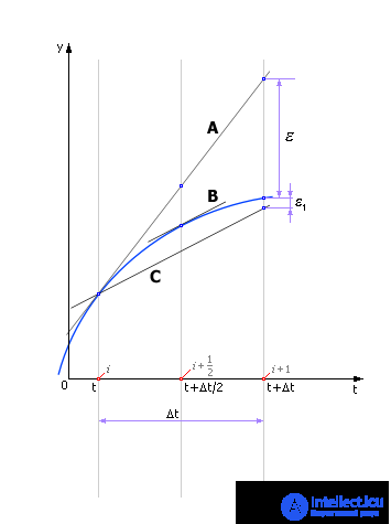
Next, transfer line B back to point t . This corresponds to the fact that from point t it is done again, - but already complete, - step Δ t to point t + Δ t in the direction corresponding to line C (Fig. 14.3). Line C is parallel to B. That is, the value of the derivative at the point t is taken artificially equal to the derivative at the point t + Δ t / 2. The calculation error (see ε 1 ) in many cases decreases in this case.
|
|
| Fig. 14.3. The movement of the real system and system, calculated by the modified Euler method, and the discrepancy between them (error). In the figure for comparison shows the result calculated by the method of Euler |
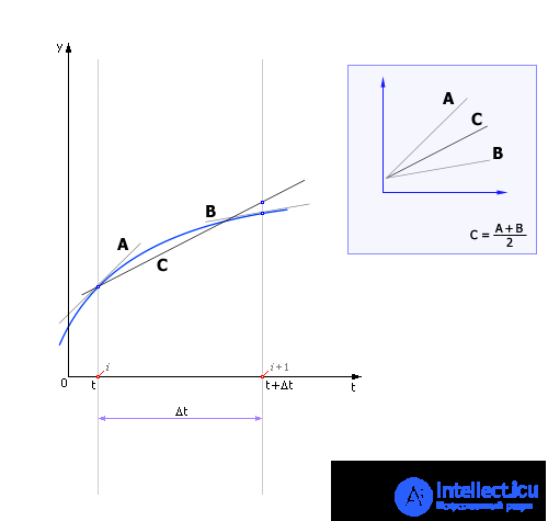
There is another variant of the modified Euler method, when the derivative in order to take a step from point i is taken not at the i -th point and not at i + 1/2, but as the arithmetic average of two derivatives: the derivative at point i (the direction of the derivative is shown in Fig. 14.4 by the line A ) and the derivative at the point i + 1 (the direction of the derivative is shown by the line B ). The direction of the “middle” derivative is shown by the line C.
|
|
| Fig. 14.4. Calculation of the movement of the system by the average derivative value in step |


Comments
To leave a comment
System modeling
Terms: System modeling