Lecture
In the process of informal synthesis, after putting forward a multitude of ideas, it is necessary to finally accept one of them for realization, since it is rather difficult to explore all the ideas in detail. To select the best (the best) of them, conduct their expertise.
For this, a team of experts analyzes the ideas, and each expert gives each idea its own assessment. The conditions for the examination are a team of experts and a list of evaluated ideas. The result of the first stage of the examination is the assessment matrix. Then, using a particular method chosen, they take into account all these estimates together and choose the best idea.
Expertise is resorted to when it is necessary to make a choice from a variety of possible ideas, solutions, projects. Examination is the expedient selection of one solution from the set of possible ones obtained at the previous stage “Generation of ideas” (see lecture 35. Informal synthesis).
There are many methods of examination: voting, ranking, pairwise comparison, the division into classes. Consider some of them.
Voting can be applied only if there are fewer opinions that are offered for consideration than those gathered.
An example illustrating this thesis is the decision of the trade union committee on the allocation of an apartment. The representative of each department of the enterprise participating in the meeting of the trade union, if he is honest, should vote only for his representative. Thus, no one will ever get the most votes. The task is simply not solved. Or it is solved by dishonest means, for example, by the collusion of two representatives alternately voting for department A, then for department B, and always winning by two votes against the rest.
The simplest way to vote is by majority vote. It has its advantages (simplicity) and disadvantages (the decision is made by an unqualified majority).
This method can be significantly improved.
Example of voting ballot. Suppose there are seven candidates for the award: Dmitriev (D), Ivanov (I), Kuznetsov (K), Lukyanov (L), Mikhailov (M), Petrov (P), Sidorov (C). The award can be received only three best. In the first round, each expert (in the example of five) evaluates each of the candidates and puts him in one place or another (see table. 36.1).
| Table 36.1. Distribution of project sites given by a team of experts (first tour) | ||||||||||||||||||||||||||||||||||||||||||||||||
|
Further points are calculated. Three experts assigned Ivanov the first place, one expert gave him the second place and one more place - the third. Knowing this, we calculate the total number of points for Ivanov: 3 · 1 + 1 · 2 + 1 · 3 = 8. In the same way, points for all other candidates are calculated. The results are tabulated (see table. 36.2).
| Table 36.2. Results of the first round | ||||||||||||||||||||||||
|
The less points a candidate has, the higher his place. This follows directly from the principle of scoring. As you can see, after the first round prizes go to Ivanov, Lukyanov and Sidorov.
After the publication of the results, there is also a lack of voting, as some experts are not satisfied with the results. For example, candidate Lukyanov (see table. 36.1), to whom none of the experts gave any of the prizes, because no one saw Lukyanov as a worthy candidate for the prize, received second place, and with it the prize. The second expert is unhappy that Sidorov entered the top three. And if he had voted again, he would have changed Sidorov and Petrov in places, forcing Sidorov to go down in the overall rating. Since there are experts interested in changing the results (by rearranging the projects), it makes sense to conduct a second round.
Let's see what the first expert will do in the second round: most likely, he will swap Petrov and Ivanov, rearrange Sidorov to second place, as his competitors Dmitriev and Kuznetsov "tread on their heels", and Ivanov, who is not threatened, will put on third place.
Other experts will do the same, but in their own way. Therefore, the voting results from round to round will change.
For example, after the second round, the rating matrix may look like this (see Table 36.3).
| Table 36.3. Distribution of project sites given by a team of experts (second round) | ||||||||||||||||||||||||||||||||||||||||||||||||
|
In addition to the results table, it is convenient to calculate the table of experts' dissatisfaction. For example, counting the sum of differences for each expert between the desired distribution of projects by location and the total result of the tour. If the expert acts logically, the rate of dissatisfaction from tour to tour, in principle, should decrease. Although it will hardly become zero, as the dissatisfaction of one expert decreases due to an increase in the dissatisfaction of another. Therefore, the procedure must come to equilibrium due to the actions of all experts simultaneously lowering their own dissatisfaction indicators.
The tour procedure continues until no expert alone can change the resulting order (result). That is, despite the fact that some experts may remain dissatisfied, they cannot change the result of the vote. Technically, this means that the result in several consecutive rounds will stop changing. His and take as an answer.
Consider the second class of examination methods.
The ranking is the ordering, the partition of the set into elements with the introduction of some order between them, in this case the order “better-worse”.
Let four experts arrange projects A, B, C and D according to rank (s), see table. 36.4.
| Table 36.4. Distribution of project sites given by a team of experts | |||||||||||||||||||||||||
|
Calculate the values of r ij - the distance between the opinions of the i- th and j- th experts. Calculate the distance between two vectors (vector - this is the opinion of an expert on a tuple of projects) can be different. Distance in mathematics is called the norm. There is the Pythagorean norm, Manhattan, Minkowski, etc. (for details, see the course “Artificial Intelligence” or “Higher Mathematics”). For example, in the matrix (see Table 36.4), we calculate the distance between the opinions of expert 1 and expert 2 in the Manhattan norm :
r 12 = | 1 - 1 | + | 2 - 3 | + | 3 - 2 | + | 4 - 4 | = 0 + 1 + 1 + 0 = 2.
So, the distance of opinions on the Manhattan norm is the sum of the differences (in absolute value) of the opinions of two experts on each project.
These values are recorded in a table (distance matrix). Then the values of R i are calculated - the distance from the i -th expert to all the others - as the sum of the distances between the opinion of this expert and other experts (see table. 36.5).
| Table 36.5. Calculation of distances between expert opinions | ||||||||||||||||||||||||||||||||||||
| ||||||||||||||||||||||||||||||||||||
Among the calculated total distances, a minimum of R i is sought. The opinion of the relevant i -th expert (with a minimum of R ) is the most average and is declared the result of the examination. Geometric interpretation shows that the opinion of this expert is located approximately in the center of a polyhedron formed by vertices, each of which represents the opinion of an individual expert, and the edges are the distances between the opinions of experts. As is known, the center is the place closest to all the vertices (opinions) of the figure at the same time.
The coordinate system for constructing a polyhedron is formed by projects. Thus, 4 projects form 4-dimensional space. The axes of the coordinates lay the points obtained by the project from this expert. Then the expert opinion is a point in the project space.
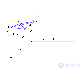
In fig. 36.1 the four-dimensional space formed by the ABCD projects is shown. To find the point - the expert's opinion - in four-dimensional space, you need to postpone along the A axis the number of points set by the expert of project A. Next, draw a line through the obtained point parallel to the next B axis and put the number of points put by the expert to project B on this line. again draw a line parallel to the C axis, putting aside the number of points supplied by the expert to the project C. And finally, draw the line parallel to D through the obtained point, putting the number of points put on it by the expert of the project D. Precise ka, corresponding to the expert's opinion in the four-dimensional space, found. It is also necessary to find points - expert opinions 2, 3, 4. Connecting the points by lines, we get a polyhedron of expert opinions.
| |
| Fig. 36.1. The polyhedron of expert opinions 1, 2, 3, 4 in the four-dimensional space of ABCD projects |
It is obvious that you can build any number of axes and reflect the space of any dimension on the plane (see Lecture 16. The concept of the dimension of space in the “Computer Graphics” discipline). What you see in fig. 36.1, there is a projection of a figure from four-dimensional space on a two-dimensional plane of the screen. Depending on how well you position the axes (more precisely, the projections of the axes) on the plane, the drawing will be more or less visual. Turning the axis, you can achieve a visual image. This is called finding a good angle for viewing a multidimensional figure. Considering rice. 36.1, note that point 1 (symbolizes the opinion of expert 1 regarding projects A, B, C, D) is closest to the opinions of other experts, unlike points 2, 3, 4. Considering a polyhedron from different sides ( turning the axis) you can make sure that the point looks from any angle. Hence, expert opinion 1 is average and is the solution.
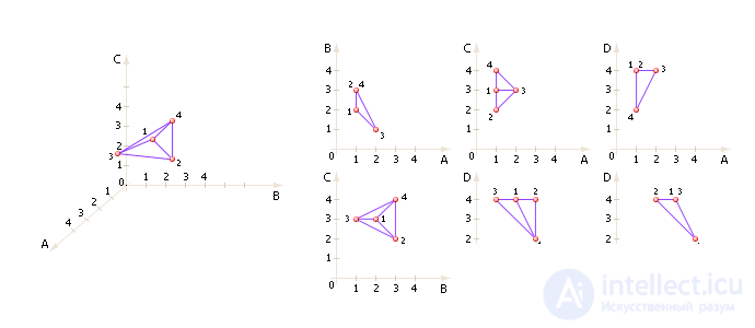
It is possible, of course, to depict this figure in three-dimensional space, and two-dimensional, and even one-dimensional or zero-dimensional (see. Fig. 36.2), which is more familiar to you. Such drawings are sections of four-dimensional space along one or two axes. This is a matter of convenience thinking. Usually, several sections are drawn at once, preferably in mutually perpendicular planes, in order to try to restore the general form of the figure for several particular types in the mind , looking at them SIMULTANEOUSLY . So do, for example, when working with drawings.
In fig. 36.2 shows a section of the four-dimensional space for three axes (A, B, C) and different pairs of two axes. (Projections on one-dimensional axes and on a zero-dimensional axis build yourself). But even from these figures it is clear that the opinion of Expert 1 is average, since it always lies inside the polyhedron (1-2-3-4).
| |
| Fig. 36.2. Projections of the polyhedron of expert opinions on the axis of ABCD projects |
Note that the most distant peak from the center characterizes the most unreliable opinion and can thus characterize the expert himself.
In our example, the distance matrix will look like this (see Table 36.6).
| Table 36.6. The calculation of the values of the distances between the opinions of experts | ||||||||||||||||||||||||||||||
|
It is obvious that expert 1 has the smallest distance from the remaining opinions, therefore his opinion is declared the result.
Answer: Project A - 1st place, Project B - 2, Project C - 3, Project D - 4. The best project is Project A.
The first place is the project to which the majority of experts assigned the first place. The second place is the project to which the majority of experts assigned the second place, and so on.
In our example (see Table 36.4), Project A will eventually take the first place, since three experts gave it the first place. Projects B and C will share the second and third places, as two experts gave them the third place. Project D will take the fourth place, as three experts gave it the fourth place.
Answer: Project A - 1st place, Project B and C share 2nd and 3rd place, Project D - 4th place. The best project is project A.
Note : you can slightly clarify the solution of the problem by resolving the dispute for 2 and 3 places in favor of project B. If you look closely, finally comparing projects B and C, the project B is more preferable than C, because it takes additional places 2 and 1, and project C only places 2 and 4.
Important note . The task answers obtained by the Kemeny Median and the majority method coincided, although this is not always the case. Solutions obtained by different methods may differ slightly from each other. But overall, the solution is stable. In some cases, individual methods may not work, so the examination is carried out with several methods, and then a general answer is derived.
Consider again our example (tab. 36.7).
| Table 36.7. Distribution of project sites given by a team of experts | |||||||||||||||||||||||||
|
First, for each pair of projects ( i and j ) we calculate what number of experts S ij thinks that the i -th project is better than j- th, and what number of S ji experts think the opposite (see table. 36.8).
| Table 36.8. Relationship calculation Better-worse between projects | ||||||||||||||||||||||||||||
|
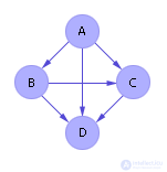
Next on the graph, arrows will show the relationship between pairs of projects (see. Fig. 36.3). The arrow from the i- th project in the column to the j- th indicates that the i- th project was preferred by more experts than the j- th. For example, the arrow from A is directed to B, since project A is better than project B (three experts preferred project B, project A, and only one expert preferred vice versa).
| |
| Fig. 36.3. Preference graph ABCD projects |
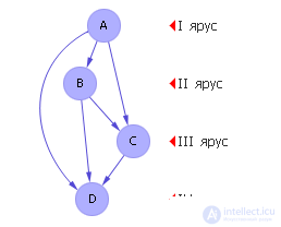
Now arrange the graph, bringing it to the tier-parallel form (JFF) (see. Fig. 36.4).
| |
| Fig. 36.4. ABCD Preference Graph in longline-parallel form |
Reduction of a graph to a YPF is its reduction to a form where there are vertices in the upper tiers, into which there are no incoming arrows from the vertices lying in the lower tiers. The algorithm for constructing the YPF graph is understood in the discipline "Discrete Mathematics". So, the YPF shows that the peak with no arrows is peak A, therefore, the absolute leader among projects is project A. Project A is better than B, it is better than C at the same time, it is better than D. Then, among the remaining projects (BCD) Project B is the best, since it is simultaneously better than C and D. And finally, C is better than D.
Answer: Project A - 1st place, Project B - 2nd place, Project C - 3rd place, Project D - 4th place. The best project is project A.
For the first place each project will give 1 point, for the second place - 2 points, for the third - 3 points and so on. Next, calculate the number of points that each project will receive in the amount. The first place in the end will receive a project that will score the smallest number of points, the remaining places will be determined by sorting the points scored.
So, for our example from tab. 34.4 we get the following (see table. 36.9).
| Table 36.9. Distribution of project sites Borda method (example) | ||||||||||||||||||||||||||||||
|
Answer: Project A - 1st place (5 points), Project B - 2nd place (9 points), Project C - 3rd place (12 points), Project D - 4th place (14 points). The best project is project A.
Рассмотрим данный метод на примере решения о покупке автомобиля.
Сначала составляют таблицу критериев, по которым будут оценивать проекты (см. табл. 36.10).
| Таблица 36.10. Таблица критериев для оценки проектов | |||||||||||||||||||||||||
|
Далее эксперт составляет таблицу оценок проектов (автомобилей). Например, для 7-ми автомобилей эксперт заполняет таблицу так, как показано в табл. 36.11.
| Таблица 36.11. Таблица оценок проектов по критериям | |||||||||||||||||||||||||||||||||||||||||||||||||
| |||||||||||||||||||||||||||||||||||||||||||||||||
Рассматриваем все пары проектов i и j . Если по какому-либо критерию i -ый проект лучше, чем j -ый, то соответствующий критерию вес прибавляется к P ij (эти баллы символизируют выбор «За»), в противном случае — к N ij (эти баллы символизируют выбор «Против»). То же самое справедливо для j -го проекта: если j -ый проект оказывается лучше, чем i -ый, то соответствующий критерию вес прибавляется к P ji , в противном случае — к N ji (обратите внимание на порядок следования индексов j и i у P и N ). Если повстречалось одинаковое для i -го и для j -го проектов значение критерия, то оно пропускается. Затем, когда по паре i и j рассмотрены все критерии, находятся отношения D ij = P ij / N ij и D ji = P ji / N ji . Значения D ≤ 1 отбрасываются. Заметим, что D ji = 1/ D ij (и наоборот), таким образом, вычисления можно несколько упростить.
Рассмотрим, для примера, проекты 2 и 4 ( i = 2, j = 4). По критерию «Цена» (вес критерия — 5 баллов) проект 2 хуже проекта 4; по критерию «Комфортность» (вес — 4 балла) проект 2 лучше проекта 4; по критерию «Скорость» (вес — 3 балла) проект 2 хуже проекта 4; по критерию «Дизайн» (вес — 3 балла) проект 2 лучше проекта 4. Таким образом, имеем:
P 24 = 0 + 4 + 0 + 3 = 7;
N 24 = 5 + 0 + 3 + 0 = 8;
D 24 = P 24 / N 24 =7/8 = 0.875 < 1 — отбрасываем;
P 42 = 5 + 0 + 3 + 0 = 8;
N 42 = 0 + 4 + 0 + 3 = 7;
D 42= P 42 / N 42 = 8/7 = 1 / 0.875 = 1.14> 1 - we accept.
Consider, for example, projects 1 and 2 ( i = 1, j = 2). According to the criterion "Price" project 1 is worse than project 2; according to the “Comfort” criterion, projects 1 and 2 are the same, so we are not doing anything; according to the “Speed” criterion, project 1 is better than project 2; according to the “Design” criterion, projects 1 and 2 are the same, therefore we do nothing. Thus, we have:
P 12 = 0 + 0 + 3 + 0 = 3;
N 12 = 5 + 0 + 0 + 0 = 5;
D 12 = P 12 / N 12 = 3/5 = 0.6 <1 - discard;
P 21 = 5 + 0 + 0 + 0 = 5;
N 21 = 0 + 0 + 3 + 0 = 3;
D 21 =P 21 / N 21 =5/3 = 1/0.6 = 1.67 > 1 — принимаем.
Все остальные пары рассчитываются аналогично.
Составляем матрицу, внося вычисленные (и принятые) значения D . Матрица имеет смысл предпочтений проектов между собой. Для нашего примера матрица выглядит следующим образом (см. табл. 36.12).
| Таблица 36.12. Полная матрица предпочтений проектов, составленная методом «Электра» | ||||||||||||||||||||||||||||||||||||||||||||||||||||||||||||||||
|
Задаемся порогом принятия решения, например C = 1.33, и оставляем в матрице те числа, которые больше или равны значению порога C . Таким образом, матрица разрежается (см. табл. 36.13).
| Table 36.13. Project preference matrix at the threshold C = 1.33 | ||||||||||||||||||||||||||||||||||||||||||||||||||||||||||||||||
|
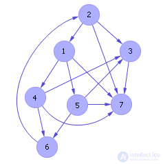
A preference graph is constructed on the matrix (see Figure 36.5). From the graph constructed on the table. 36.13, it is clear that project 1 is better than projects 4, 5, 7; project 2 is better than projects 1, 3, 7; project 3 is better than project 7; project 4 is better than projects 3, 6, 7; project 5 is better than projects 3, 6, 7; project 6 is better than project 2.
| |
| Fig.36.5. Type of preference graph for the case of a decision threshold C = 1.33 |
Очевидно, что решение не получено, так как в графе присутствуют петли. Например, 2 лучше 1, 1 лучше 5, 5 лучше 6, 6 лучше 2. Назначим порог отбора предпочтений C = 1.4 (это соответствует тому, что мы попробуем учесть только более сильные связи в графе, не отвлекаясь на малозначимые расхождения в проектах). Таким образом, матрица еще разрежается. В ней остаются только самые сильные связи (см. табл. 36.14).
| Таблица 36.14. Матрица предпочтений проектов при пороге C = 1.4 | ||||||||||||||||||||||||||||||||||||||||||||||||||||||||||||||||
|
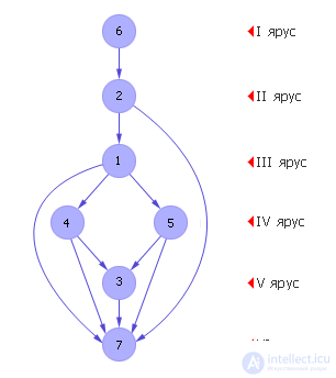
По матрице строится граф предпочтений (см. рис. 36.6). По графу и табл. 36.14 видно, что проект 1 лучше проектов 4, 5, 7; проект 2 лучше проектов 1, 7; проект 3 лучше проекта 7; проект 4 лучше проектов 3, 7; проект 5 лучше проектов 3, 7; проект 6 лучше проекта 2. Как видим из рис. 36.6, при C = 1.4 граф получился в таком виде, в котором он легко приводится к ЯПФ, следовательно, решение получено.
| |
| Fig. 36.6. Вид графа предпочтений для случая порога принятия решений C = 1.4 |
Петель в графе нет, при этом граф остался целостным. Решение говорит нам о том, что лучший проект — 6. На втором месте — проект 2, на третьем месте — проект 1, четвертое и пятое место делят проекты 4 и 5, на шестом месте — проект 3, на седьмом месте — проект 7.
Notes
| |
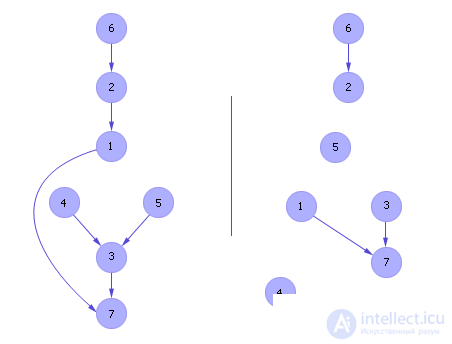
| Fig. 36.7. Вид графа предпочтений для случая порога принятия решений C = 1.67 (слева) и C = 2 (справа) |
Важным вопросом экспертизы является формирование группы экспертов. Если экспертов много, то в группу с высокой вероятностью попадают некомпетентные эксперты. Если экспертов мало, то результат экспертизы существенно зависит от конкретных лиц, попавших в число экспертов. Поэтому имеет смысл, опросив экспертов r i и получив результат экспертизы R , оценить объективность каждого из членов экспертного коллектива по следующей формуле:

|
Для нашего примера можно просчитать объективность каждого эксперта. Рассмотрим уже полученное ранее решение (см. табл. 36.15).
| Таблица 36.15. Матрица мнений экспертов и результат экспертизы | ||||||||||||||||||||||||||||||
|
Расстояние d ( r i , R ) от мнения i -го эксперта до результата (среднего мнения R ):
d ( r 1 , R ) = |1 – 1| + |2 – 2| + |3 – 3| + |4 – 4| = 0;
d ( r 2 , R ) = |1 – 1| + |3 – 2| + |2 – 3| + |4 – 4| = 2;
d ( r 3 , R ) = |2 – 1| + |1 – 2| + |3 – 3| + |4 – 4| = 2;
d ( r 4 , R ) = |1 – 1| + |3 – 2| + |4 – 3| + |2 – 4| = 4.  = 0 + 2 + 2 + 4 = 8.
α 1 = 1 – 0/8 = 1;
α 2 = 1 – 2/8 = 0.75;
α 3 = 1 – 2/8 = 0.75;
α 4 = 1 – 4/8 = 0.5.
Итак, как видим, первый эксперт имеет наибольшую объективность; наименьшую объективность имеет четвертый эксперт (см. рис. 36.8). Кстати, неслучайно в методе «Медиана Кемени» мнение первого эксперта было принято в качестве ответа экспертизы, а четвертый эксперт стоял на периферии многоугольника мнений экспертов ABCD (см. рис. 36.1 и рис. 36.2)…
| |
| Fig. 36.8. Диаграмма объективности экспертов |
In general, it is recommended to weed out the opinions of experts with a small value of α and recalculate the result R without taking them into account.
The second expert review concerns the consistency of their team. To calculate the consistency of opinions, we calculate the variance of opinions (see Table 36.16) and estimate its value by the statistical formula W = 12 · D / ( n 2 · ( m 3 - m )), where n is the number of experts, m is the number of projects.
| Table 36.16. Matrix for calculating the consistency of opinions experts for a group of four experts | ||||||||||||||||||||||||||||||||||||||||||||||||||||||||
|
For our case, we have: W = 12 · 46 / (4 2 · (4 3 - 4)) = 552/960 = 0.575. With W = 1, the experts are in complete agreement; at W = 0, there is a complete inconsistency. In our example, expert consensus is weak. Therefore, it may be recommended to change the number of experts - either remove the fourth expert as the most biased, or increase the number of experts for more statistical stability of the results. Let's see how the consistency of experts will increase, for example, after the removal of the fourth expert (see table. 36.17).
| Table 36.17. Matrix for calculating the consistency of opinions experts for a group of three experts | |||||||||||||||||||||||||||||||||||||||||||||||||
|
W = 12 · 29 / (3 2 · (4 3 - 4)) = 0.64 - as we see, the agreement has increased.
Thus, the expertise helps us to conduct an informal analysis in modeling, selecting the most promising version of the future project from among the many methods proposed by generating ideas. Subsequently, significant funds will be invested in the selected project for its detailed elaboration (design and modeling process - see lecture 01. Modeling concept. Methods for presenting models and Fig. 1.14. Diagram of the process, modeling methods and techniques (full version)).
Usually, for confident decision making, since all the methods of expertise are subjective, several methods are used at once and a general solution is derived.
The resulting solution must be checked. We reviewed two checks - on the quality of the expert (objectivity of the expert) and the quality of the group (group consistency).
The very value of the criterion obtained as a result of the test gives only a relative estimate. It is recommended to observe a change in magnitude as a result of a change in some significant factor and to achieve the best value of this quantity, consciously controlling this factor (see, for example, table 36.16 and table 36.17). Such a factor can most often be the size of the group, the qualitative composition of the expert group, the system of criteria, the composition of projects. Good results are obtained by the use of iterations in the examination.
But it should always be borne in mind that no number of checks, even very large ones, guarantee the absolute correctness of the choice of the solution.
 — сумма расстояний от всех мнений экспертов до среднего мнения R .
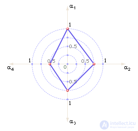

Comments
To leave a comment
System modeling
Terms: System modeling