Lecture
The main neural network paradigms were developed several decades ago, according to their research, a huge number of papers were published with reviews that can be found in [1–4]. We only, for a better understanding of the further architectural and circuit design solutions of neural computing systems, will dwell on the most important elements of neurology from the standpoint of hardware implementation.
One of the main advantages of the neurocalculator is that its basis is made up of relatively simple, most often - of the same type, elements (cells) that imitate the work of brain neurons - "neurons". Each neuron is characterized by its current state, by analogy with the nerve cells of the brain, which can be excited or inhibited. It has a group of synapses - unidirectional input connections connected to the outputs of other neurons, and also has an axon - output connection of a given neuron, with which a signal (excitation or inhibition) enters the synapses of the following neurons. A general view of the neuron is shown in Figure 2.
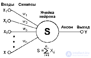
Fig.2. General view of the neuron.
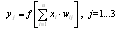
Each synapse is characterized by a synaptic connection or its weight w i , which is physically equivalent to electrical conductivity. The current state of a neuron is defined as the weighted sum of its inputs:

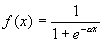
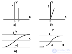
The output of a neuron is a function of its state: y = f (s) (2), which is called activation and can have a different form (some of the typical activation functions are presented in Figure 3). One of the most common is a non-linear function with saturation, the so-called logistic function or sigmoid (i.e., S-shaped function):
Pic2.5
a) a single threshold function;
b) linear threshold (hysteresis);
c) sigmoid - hyperbolic tangent;
d) logistic sigmoid.
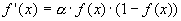
While decreasing  sigmoid becomes flatter, in the limit at = 0 degenerating into a horizontal line at 0.5, with increasing the sigmoid approaches in appearance to the function of a single jump with a threshold T at the point x = 0. From the expression for sigmoid it is obvious that the output value of the neuron lies in the range [0,1]. One of the valuable properties of a sigmoid function is a simple expression for its derivative.
Parallelism of processing is achieved by combining a large number of neurons into layers and connecting in a certain way different neurons among themselves. As an example of the simplest NA, we give three neural perceptrons (Fig. 3), whose neurons have an activation function in the form of a single threshold function, the work of which is discussed in detail in the literature [2-4]. At the n inputs, there are some signals passing through synapses into 3 neurons, forming a single layer of this NA and producing three output signals:
Obviously, all the weights of synapses of a single layer of neurons can be reduced to a matrix W, in which each element w ij specifies the value of the i-th synaptic connection of the j-th neuron. Thus, the process occurring in the NA can be written in the matrix form: Y = F (XW), where X and Y are the input and output signal vectors, respectively, F (V) is the activation function applied elementwise to the components of the vector V. Theoretically, the number of layers and the number of neurons in each layer can be arbitrary.
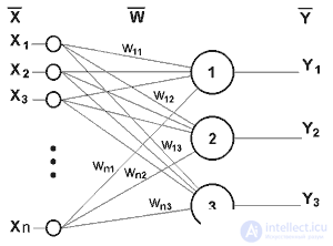
Fig.3 Single-layer perceptron.
In order for the neural network to work, it must be trained. The ability of the network to solve the problems set before it depends on the quality of training. At the training stage, in addition to the quality parameter for selecting weighting factors, the training time plays an important role. As a rule, these two parameters are inversely related and they have to be chosen on the basis of a compromise. NA training can be conducted with or without a teacher. In the first case, the network presents the values of both the input and the desired output signals, and it adjusts the weights of its synaptic connections by some internal algorithm. In the second case, the outputs of the NA are formed independently, and the weights are changed according to an algorithm that takes into account only the input signals and their derivatives.
Considering the classification of NAs, one can distinguish: binary (digital) and analogue NA, pre-trained (non-adaptive) and self-learning (adaptive) neural networks, which is extremely important when implementing them in hardware. Binary operate with binary signals, and the output of each neuron can take only two values: a logical zero ("inhibited" state) and a logical unit ("excited" state). The three neural perceptron considered above also belongs to this class of networks, since the outputs of its neurons, generated by the single hop function, are either 0 or 1. In analog networks, the output values of neurons can take continuous values, which could occur after replacing the activation function perceptron neurons on sigmoid.
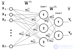
Fig. 4. Two-layer perceptron
Networks can also be classified by topology (the number of layers and the connections between them). Figure 4 shows a two-layer perceptron derived from the perceptron of Figure 3 by adding a second layer consisting of two neurons. In this case, the nonlinearity of the activation function has a specific meaning: since if it did not have this property or did not belong to the algorithm of each neuron, the result of the operation of any p-layer NS with weight matrices W (i) , i = 1,2 ,. ..p for each layer i would be reduced to multiplying the input vector of signals X by the matrix W (  ) = W (1) ..W (2) W ... CH (p), that is, in fact, such a p-layer HC is equivalent to a single-layer HC with a weight matrix of a single layer W ( ): Y = XW ( ).
There are a great many different learning algorithms that are divided into two large classes: deterministic and stochastic. In the first of these, the adjustment of the weights is a rigid sequence of actions; in the second, it is carried out on the basis of actions that obey a random process.
Almost 80% of neurochips implemented for today, focused on digital signal processing, use the back propagation error algorithm when teaching NS, among other things, it has become a kind of benchmark for measuring the performance of neural calculators (for example, as an FFT 1024 samples for signal processors), therefore it is worth staying in more detail.
Consider this algorithm in the traditional formulation [1-4]. It represents the propagation of error signals from the outputs of the NA to its inputs, in the direction opposite to the direct propagation of signals in normal operation. This learning algorithm is called the National Assembly back propagation procedure (Back Propagation). According to the method of least squares, the minimized objective function of the error of the NA is the signal of the training error:
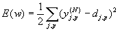
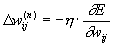
Where  - the real output state of the neuron j of the output layer N of the neural network when the pth image is applied to its inputs; d jp is the ideal (desired) output state of this neuron. Summation is performed over all neurons of the output layer and over all images processed by the network. Minimization is carried out by the method of gradient descent, which means the adjustment of the weighting factors as follows:
Here w ij is the weighting factor of the synaptic connection connecting the i-th neuron of the n-1 layer with the j-th neuron of the n layer,  - learning rate coefficient, 0 < <1.
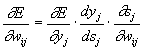
Here, y j , as before, means the output of the neuron j, and s j is the weighted sum of its input signals, that is, the argument of the activation function. Since the factor dy j / ds j is a derivative of this function with respect to its argument, it follows from this that the derivative of the activation function must be defined on the entire x-axis, i.e. they use smooth functions such as hyperbolic tangent or classical sigmoid with an exponent. In the case of hyperbolic tangent

The third factor s j / w ij is obviously equal to the output of the neuron of the previous layer yi (n-1) ; to express the derivative of the error signal with respect to the output signal, we have:
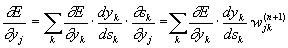
Here, summation over k is performed among the neurons of the layer n + 1.
Entering a new variable
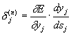
we get a recursive formula for calculating  j (n) of layer n of values k (n + 1) of the higher layer n + 1.
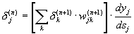
For the same output layer
Now we can write the main expression for the weights in a generalized form:
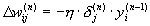
Sometimes, in order to impart a certain inertia to the correction process of the weights, smoothing out sharp jumps when moving over the target function, the value of the weight change at the previous iteration is added (that is, we have already come close to the well-known adaptive LMS algorithm).

Where  - coefficient of inertia, t - number of the current iteration.
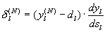
Figure 5 shows a diagram of signals in the network when learning using the reverse propagation algorithm. It structurally reflects all neural network operations and visually illustrates those structural and functional elements that should be implemented in the unit cell of the neurocalculator.
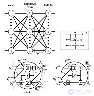
Fig.5. Diagram of signals in the network when training on the back propagation algorithm [3]
Considered NA has a number of shortcomings [1-4]: Firstly, in the learning process, a situation may arise when large positive or negative values of weight coefficients shift the working point on the sigmoids of many neurons to the saturation region. Small values of the derivative of the logistic function will lead to the cessation of training, which paralyzes the NA. Secondly, the use of the gradient descent method does not guarantee that a global minimum, rather than a local minimum, of the objective function will be found. This problem is connected with one more, namely with the choice of the magnitude of the learning rate. Proof of convergence of learning in the process of backward propagation is based on derivatives, that is, the increments of weights and, therefore, the learning rate must be infinitely small, but in this case learning will be unacceptably slow. On the other hand, too large corrections of weights can lead to a constant instability of the learning process. Therefore, as usually a number less than 1 is chosen, but not very small, for example, 0.1, and, generally speaking, it can gradually decrease in the learning process. In addition, to exclude random hits to local minima, sometimes, after the values of the weighting factors are stabilized, temporarily increase greatly to begin a gradient descent from a new point. If repeating this procedure several times will bring the algorithm to the same state of the NA, you can more or less confidently say that a global maximum has been found, and not some other.
Another simple example is the construction of a neuroadaptive control system on delay lines. In this case, the neurocalculator can be implemented on the basis of adaptive adders (transversal filters, for example, on the basis of IC A100), while the presence of nonlinearity at the output of neurons is not required. The structural diagram of such a neural system for the one-dimensional case and processing in the time domain, shown in Fig.6, consists of five layers, the input signals of neurons of 2-4 layers form the shift registers RG, the length of which determines the order of the control system. The neurons of layers 1 and 5 only sum the input signals. The neurons of the second layer take into account changes in the characteristics of the control object in the area from the meter to the controller, for which a generator uncorrelated with the input signal is introduced into the circuit. The third layer of the neural network performs the formation of the control signal, and the fourth takes into account the influence of the regulator on the primary meters. Such a construction of a one-dimensional control system allows you to organize a five-level pipeline, and the proposed approach to adjusting the weight coefficients makes it possible to abandon the classical back-propagation procedure for training a neural network and use neurons without non-linear elements at the outputs.
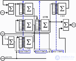
Fig.6. Block diagram of a one-dimensional neuroadaptive control system on delay lines.
The algorithm of the neuroadaptive control system of such a structure is as follows.
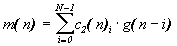
The first layer: g (n) = x (n) -q (n-1), e 1 (n) = e (n) -v (n-1). Second layer: c 2 (n) i = c 2 (n-1) i -
The third layer: h (n) i = h (n-1) i -Fourth layer: c 1 (n) i = c 1 (n-1) i -
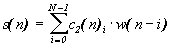
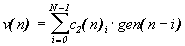
The fifth layer: y (n) = w (n) + gen (n).
Where x (n) is the sequence of input signals, y (n) is the sequence of compensation signals, e (n) is the error signal of compensation, w (n), e 1 (n), s (n), g (n), q (n), v (n) - intermediate signals, gen (n) - generator signal sequence, h (n), c 1 (n), c 2 (n) - weighting factors. The transition to a control system of a higher spatial dimension can be accomplished by cascading one-type neuromodules of the same type, similar to that shown in Figure 6. In this case, the neurons of the first layer will also be endowed with the properties of a weighted summation of the input signals from the sensors, and the values of the weighting factors will take into account the mutual correlation between the sensors.
Hardware this system can be implemented on the basis of Texas Instruments TMS320C32-60 32-bit DSP with 24-bit address bus and performance up to 60 ml. floating point operations per second (the execution time of the complex Fourier transform for a frame of 1024 samples is about 1.6 ms). This processor has the Neumann architecture (the total address space for the executable code and data) and provides two floating point operations in one machine cycle and has the ability to simultaneously perform input / output operations. High speed is provided by parallel processing and large internal memory (two banks of internal RAM 256x32 + Cache 64x32 commands). Все команды процессора имеют фиксированную длину в 32 бита при этом имеется возможность выполнения параллельных команд за один машинный цикл, что позволяет реализовывать нейросетевые алгоритмы (однако выигрыш в производительности от использования нейроалгоритмов меньше, чем при мультипроцессорной архитектуре). Для данной реализации участок листинга программы нахождения вектора весовых коэффициентов центрального узла настройки системы управления приведен в таблице 2.
Табл.3. Участок листинга алгоритма обучения.
Участок листинга алгоритма обучения
  ....
 ; AR0 - адрес регистра с имп. хар. h(N-1),
 AR1 - адрес регистра со значениями x(n-N+1), RC регистр счетчика
 ; со значением равным N-2, BK - регистр циклической адресации со значением равным N.

MPYF3 *AR0++(1),*AR1++(1)%,R1 ;перемножаем два плав. числа и результат заносим
                                 ;в регистр повышенной точности R1 (float -40 бит).
LDF 0.0, R0 ;загружаем плав. число 0.0 в рег. R0 - инициализация
RPTS RC ;Начало цикла (RC - 32 битный регистр счетчика)
MPYF3 *AR0++(1),*AR1++(1)%,R1||ADDF3 R1,R0,R0
                                 ;параллельно за один машинный цикл осуществляем
                                 ;умножение и сложение чисел. (выполняем N-1 раз)
ADDF R1,R0,R1 ;производим последнее суммирование в цикле
 ........
RETS ;  Output
Данный участок листинга программы работы нейроадаптивной системы управления занимает шесть 32-битовых слов с временем выполнения TЦУН = 32*(11+(N-1)) (нс), для узла настройки с N=160 это займет: TЦУН = 32*(11+(N-1)) = 32*(11 + 159) = 5440 нс.
Выигрыш при использовании нейросетевого подхода, по сравнению с традиционным, заключается в том, что возможно проводить вычисления параллельно, а это в свою очередь дает возможность реализовать системы управления более высокого порядка при приемлемых показателях сходимости и, следовательно, добиться более высокого качества управления. Нейросетевой подход к реализации многомерных пространственных систем управления во многом снимает проблемы стоявшие перед разработчиками по необходимости выполнения векторно-матричных операций высокой размерности в реальном времени.
Кроме многослойных нейронных сетей обратного распространения, основной недостаток которых - это невозможность гарантировать наилучшее обучение за конкретный временной интервал, на сегодня известно достаточно большое количество других вариантов построения нейронных сетей с использованием разнообразных нейросетевых алгоритмов, однако и они имеют как определенные преимущества, так и специфические недостатки. Всё это делает актуальным решение конкретных теоретических и практических задач применения нейросетевых технологий для различных областей, чему, мы надеемся, будут способствовать материалы данного и последующих обзоров.
В общем случае проектирование нейросистем сложный и трудоемкий процесс, в котором выбор конкретного алгоритма - это только один из нескольких шагов процесса проектирования. Он, как правило, включает: исследование предметной области, структурно-функциональное проектирование, топологическое проектирование и т.д. В качестве примера на рис.7. приведена часть алгоритма проектирования нейросетевого блока управления микропроцессорной системы активного управления волновыми полями (в данном случае акустическим [8]).
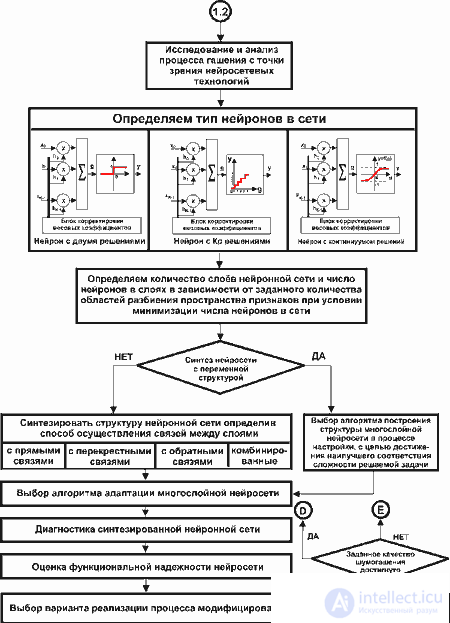
Fig.7. Алгоритм проектирования нейроадаптивной системы активного управления акустическим полем.
Вопросы, стоящие перед разработчиками нейросетевой элементной базы и нейровычислителей, во многом сложны и требуют дополнительных исследований: как целесообразней реализовать нейрочип - со встроенными нелинейными преобразованиями (пусть и фиксированного набора, но реализованных аппаратно) или позволить программисту - разработчику нейронной сети, самому формировать активационную функцию программно (размещая соответствующий код в ПЗУ). Стоит ли гнаться за универсальностью нейрочипа, которая позволила бы реализовывать любые топологии и парадигмы, или следует ориентироваться на выпуск специализированных предметно ориентированных нейрочипов, использовать ли базовые матричные кристаллы (БМК) и ПЛИС: все эти вопросы требуют ответа (по крайней мере обсуждения). Мы предлагаем всем заинтересованным лицам продолжить данное обсуждение в on-line форуме на сервере "Новости с Российского рынка нейрокомпьютеров" (http://neurnews.iu4.bmstu.ru).
В заключении подчеркнем, что эффективное применение нейрокомпьютеров характерно для случаев, требующих резкого сокращения времени обработки при решении пространственных задач повышенной размерности, которых можно найти множество практически в любой области деятельности. В следующих разделам мы подробнее остановимся на элементной базе нейровычислителей и архитектуре их построения.

Comments
To leave a comment
Computer circuitry and computer architecture
Terms: Computer circuitry and computer architecture