Flat linear surface wave antennas.

1. Antennas with a dielectric guide. Consider the antenna shown in Fig. 14.2. We assume that the length of the protruding part of the screen is outside the guide. Let the relative dielectric constant of the guide is equal to e _G.

Fig. 14.2. Flat linear surface wave antenna.

E- type waves , as is known from the theory of the electromagnetic field [1], can propagate along the direction, if in the aperture of the exciting horn the electric vector is parallel to the y axis. If the thickness of the guide h < , then only the wave of type E ₀ will propagate (Fig.14.3, a), which does not have a critical wavelength. The field amplitude will decrease exponentially in the direction of the Oy axis (Figure 14.3, b). The Eo type wave has two components: Ey and E Z. The surface wave will propagate along the axis O z with a phase velocity v _f , which can be determined from the transcendental equation:

, (14.1)

where is the deceleration factor x = c / v f . If kh > 0, then x < 1 and v _{Ф >} c . If kh grows, then x < and v _F = c / . Thus, the phase velocity is within: c / > v _{F <} with.

Neglecting radiation from the side and end walls of the sender, it is possible in the first approximation to assume that the antenna has a radiating aperture with dimensions L and a. The amplitude-phase distribution in this opening can be approximately considered as separable. Along the Oz axis, the phase changes according to the law of a traveling wave, and the amplitude in the first approximation can be considered constant (if the losses in the dielectric and in the substrate are small). Along the axis Ox, the field distribution is the same as in the exciter.

Fig. 14.3. The structure of the field wave type E ₀ (a);

a decrease in the component Ey along the coordinate y (b).

It follows from the above that the antenna DN in the yOz plane (E-plane) depends only on the longitudinal size L and, according to the diagram multiplication theorem, can be represented as:

f ( q ) = f o ( q ) f _C ( q ). (14.2)

Here f о ( q ) is the elementary radiation source of the elementary radiator, as which one can take a strip of length dz (see Fig. 14.2). Since the tangential component of the electric field is oriented along the Oz axis (perpendicular to the edges of the strip) on the surface of the guide, such a strip can be considered as a rectilinear gap for which in the Е-plane fo ( q ) = 1 (see §10.3); f _С ( q ) - DN of continuous rectilinear equal amplitude system of axial radiation. As shown earlier (see §3.4),

, (14.3)

Since x > 1, the main lobe of the DN is oriented along the axis Oz. DN has a form typical of axial radiation antennas. To assess the shape of the pattern, one can refer to Fig. 3.12, in which, however, because of the infinite length of the metal screen, only the upper half of the pattern makes sense.

Formula (14.3) was obtained under the assumption that the thickness of the guide does not vary along the length of the antenna, i.e. x = const. In fact, to match the antenna with free space, its thickness is reduced to the end (dotted lines in Figure 14.2). In this case, the average value of x along the antenna length should be substituted into formula (14.3) .

The optimal length of the antenna (at which the directivity factor is maximal) is determined by the formula (3.63)

L _OPT = l / 2 ( x -1). (14.4)

The antenna pattern in the xOz plane (H-plane) is also determined by the formula (14.2), in which the fo ( q ) should be understood as the DN of a strip of width a and length dz , but now in the H plane , i.e. fo ( q ) there is a DN of the pathogen in the H plane , since the size and amplitude-phase distribution along the Ox axis of the strip and the pathogen are the same.

Fig. 14.4. DN antenna surface waves in the plane,

perpendicular to the screen.

With real antennas, the screen length is not infinite. At the edge of the screen, the waves are diffracted, which affects the shape of the NAM. If La = 0, then to calculate the DN in the illuminated half-space, formula (14.2) is applicable, but good agreement between the calculated and experimental DNs is obtained if in formula (14.2 ) we understand fo ( q ) as the DN of a Huygens radiator located in the aperture of the antenna . It can be shown [2] that

. (14.5)

Since the maxima of the functions f о ( q ) and f с ( q ) take place respectively at angles q = 90 ° n q = 0, the main lobe of the DN is deflected from the screen by a certain angle, which is smaller, the longer the antenna and the more slow down x . A typical DN is shown in Fig. 14.4. Some radiation is observed in the shaded half-space (below the screen).

If L = 0, then to determine the radiation field, it is necessary to take into account the radiation of currents flowing around the protruding part of the screen, which greatly complicates the calculation [2].

Type H waves will propagate along a guide when the electric vector of the field in the aperture of the pathogen (see Fig. 14.2) is parallel to the axis Ox. In order to propagate only the main magnetic wave of type But, it is necessary to fulfill the condition: .

Unlike a wave of type E o, a wave of type H o has a critical wavelength, therefore, in order for wave But to exist, it is necessary to fulfill the condition: .

The calculation of the radiation field of the antenna in the case of a wave of type But is the same as in the case of a wave of type Eo. The difference between the two antennas is that in the case of the But type wave, not only with the finite screen length, but also with its infinite length, the main lobe is deflected from the screen plane. This is explained by the fact that the tangential component of the electric vector in the aperture of the antenna is parallel to the axis Ox (see Fig. 14.2) and, therefore, the DN of the elementary radiator in the yOz plane must be calculated as for an elementary gap in the H- plane using the formula sin q .

Thus, there is no radiation along the screen (for q = 0) in the case of a Ho type wave.

2 Antennas with ribbed guide. It is known from the electromagnetic field theory [1] that surface waves of type E can propagate along a ribbed structure. The main wave of type Ео is of the greatest interest, the structure of which is similar to the structure of a wave of type Ео propagating above a dielectric moderator (see Fig. 14.3).

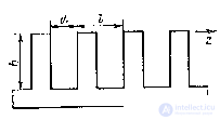
Fig. 14.5. Ribbed structure.

Fig. 14.6. The dependence of the reciprocal of the deceleration coefficient (1 / x = v _f / s) on the parameters of the ribbed structure.

The condition for the existence of a surface wave has the form: l < l / 2 x , where l is the period of the ribbed structure (Figure 14.5). A surface wave of type Eo propagates in the direction of the z axis , perpendicular to the edges, with a phase velocity that can be approximately determined by the formula:

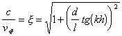, (14.6)

where h and d are respectively the depth and width of the grooves.

From formula (14.6), it can be seen that with increasing depth of the groove the phase velocity decreases and, at h = l / 4, it is zero, which corresponds to a breakdown in the propagation of the surface wave. A detailed analysis shows [1] that the ratio h / l , at which a breakdown occurs, depends on the “density” of the structure, i.e. the ratio h / l .

The results of the calculation of the phase velocity of the Eo type wave propagating along the ribbed structure are shown in Fig. 14.6. The breaks in the curves correspond to the breakdown of the surface wave.

With a known phase velocity, the calculation of the directional properties of the ribbed antennas is no different from the calculation of antennas with a dielectric guide.