Lecture
1.3.1 General Information
A measurement can be considered complete if not only the measurement result is found, but also an estimate of its error is made. In metrology, the definition of “error” is one of the central ones, and it reflects the concepts of “measurement result error” and “measurement tool error”. These two concepts are close to each other and are usually classified according to the same characteristics.
The error of the measurement result is the deviation of the found value from the true value of the measured value. Since the true value of the measured quantity is unknown, then, when quantifying the error, the actual value of the physical quantity is used . This value is found experimentally and so close to the true value that it can be used instead of it for the stated measurement task.
The error of the measuring instrument is the difference between the readings of the measuring instrument and the true (valid) value of the measured physical quantity. It characterizes the accuracy of the measurement results of the used tool.
The form of quantitative expression of the error is divided into absolute, relative and reduced.
The absolute error Δ, expressed in units of the measured value, is the deviation of the measurement result A from the true value of X.
Δ = A - X, (1.7)
A variation of the absolute error is the marginal error Δt — an error that cannot be greater than this measurement experiment.
Absolute error characterizes the value and sign of the error obtained, but does not determine the quality of the measurement itself. The characteristic of measurement quality is measurement accuracy , reflecting the measure of closeness of the measurement result to the true value of the measured value. The high accuracy of measurements corresponds to a small error. For example, the measurement of the current strength of 10 and 100 A can be performed with identical absolute error A = ± 1 A. However, the quality of the first measurement is worse than the second. Therefore, to compare the quality of measurements, use the relative error.
The relative error δ is the ratio of the absolute measurement error to the true value of the measured value:
δ = Δ / X, (1.8)
A measure of measurement accuracy is the indicator, the inverse of the module relative error: CT - 1 / | δ |. The relative error δ is often expressed as a percentage:
δ = 100Δ / X%
Since usually Δ << X, then the relative error can be defined as δ << Δ / A or δ ≈ 100Δ / A%.
The reduced error γ, which expresses the potential accuracy of measurements, is the ratio of the absolute error Δ to some normalizing value XN (for example, to the final value of the scale):
γ = 100  ∆%
∆%
X N (1.9)
By the nature (patterns) of the manifestation of the error is divided into three main classes: systematic, random and gross (blunders).
Systematic errors Δс are the components of measurement errors that remain constant or change regularly during repeated measurements of the value under the same conditions. Such errors reveal a detailed analysis of their possible sources and reduce the introduction of an appropriate amendment, the use of more accurate instruments, calibration of instruments using working measures, etc.
0
Random errors ∆ are the components of measurement errors, varying randomly in meaning and sign when repeated measurements of the same physical quantity in the same conditions. These errors appear when repeated measurements of the same physical quantity in the form of some variation in the results obtained. Description and estimation of random errors are possible only on the basis of probability theory and mathematical statistics.
Rough errors (blunders) - errors that significantly exceed those expected under given measurement conditions. They occur due to operator errors or unaccounted external influences. In the case of a single measurement can not detect a miss. With repeated observations, misses are detected and excluded in the process of processing the results of observations.
So, if you do not take into account the blunders, the absolute measurement error Δ defined by expression (2.1) is the sum of the systematic and random components:
0
∆ = ∆ s + ∆, (1.10)
The absolute error means, as well as the measurement result is a random variable.
For the reasons for the occurrence of error, measurements are divided into methodological, instrumental, external, and subjective (personal).
Methodical errors arise due to the imperfection of the measurement method, the incorrectness of the algorithms or formulas by which the measurement results are calculated, due to the influence of the selected measurement tool on the measured parameters of signals, etc.
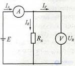
Figure 1.3 For example 2.1
Example 2.1 Let us analyze the appearance of a methodical error in measuring the resistance by the method of a voltmeter-ammeter (Fig. 2.1). To determine the value of the resistance Rx of the resistor, it is necessary to measure the current 1R flowing through the resistor and the voltage drop across it UR. In the above scheme that implements this method, the voltage drop across the resistor is measured by a voltmeter directly, while the ammeter measures the total current, one part of which flows through the resistor, the other part through the voltmeter. As a result, the measured resistance value will not be RX = UR / IR but R '= URI (IR + Iy), and a methodical error ΔR = R' - RX, will appear. Methodical error decreases and tends to zero. At current IV → 0, i.e. when the internal resistance of the voltmeter RV → ∞.
Instrumental (instrumental) errors arise due to the imperfection of measuring instruments , i.e. from their errors. Reduce instrumental errors using a more accurate instrument.
External errors are associated with the deviation of one or several influencing quantities from normal values or their output outside the normal region.
Subjective errors are caused by operator errors when reading readings (errors from negligence and operator neglect).
By the nature of the behavior of the measured value in the measurement process , static and dynamic errors are distinguished.
Static errors occur when measuring the steady-state value of the measured value.
Dynamic errors occur in dynamic measurements, when the measured physical quantity varies with time. The reason for the appearance of dynamic errors is the discrepancy between the speed (temporal) characteristics of the device and the rate of change of the measured value.
According to the operating conditions, the measuring instruments distinguish between the main and additional errors.
The main error of measuring instruments occurs under normal operating conditions specified in the regulatory documents.
Additional error of measuring instruments arises due to the output of any of the influencing quantities outside the normal range of values.
1.3.2 Accuracy classes of measuring instruments
In measurements in everyday life, increased accuracy is not always necessary. However, certain information about the possible instrumental component of the measurement error is necessary and therefore it should be reflected in some way. Such information is contained in the indication of the accuracy class of the measuring instrument.
Accuracy class is a generalized characteristic of a measuring instrument, determined by the limits of permissible basic and additional errors, as well as other properties of measuring instruments that affect the accuracy, the values of which are established in the relevant standards. It may be noted such a note: "The accuracy class of measuring instruments characterizes their properties in terms of accuracy, but is not a direct indicator of the accuracy of measurements made using these means."
Accuracy classes are assigned to measurement tools when developing on the basis of research and testing of a representative batch of such devices. Usually they are installed in the technical conditions on the measuring instrument. The limits of permissible errors are normalized and expressed in the form of absolute (∆si = ∆), relative (δsi = δ) or reduced (γci = γ) errors (hereafter, the “si” index is omitted for simplicity). The form of the expression depends on the nature of the change in the errors within the measurement range, as well as on the conditions of use and purpose of the measuring instrument.
The absolute error of measuring instruments ΔSI = Δ consists of additive (summable with the measured value) and multiplicative (multiplied by the measured value) components. The additive component is formed, for example, due to the inaccuracy of zeroing before measurement, etc. Multiplicative errors appear due to changes in the gain of the amplifier, the transmission coefficient of the circuit.
1.3.3 General information on the processing of measurement results
Due to the influence of numerous and fundamentally unrecoverable factors causing random errors, the result of each measurement Ai will differ from the true value X of the measured value: Аi - X = ΔXi. This difference is called the random error of a single measurement.
The true value of X is unknown to us. However, after a large number of measurements of the quantity X under study, the following statistical patterns can be identified:
1) If we conduct a series of measurements of the quantity being studied and determine the average value, then the positive and negative deviations of individual measurement results from the average value have an approximately equal probability. This is the reason that there is an equal probability (frequency) of the deviation of the measurement results from the true value of the magnitude in the direction of decreasing and increasing, in the case when the systematic error is zero.
The arithmetic average calculated on the basis of a series of measurements is the most reliable value that can be attributed to the measured value. When calculating the arithmetic mean of a large number of measurements, the errors of individual measurements that have a different sign are mutually compensated.
2) The probability (frequency) of the occurrence of large deviations from the result obtained is much less than the probability (frequency) of the appearance of small deviations. These statistical patterns are valid only with repeated measurements repeated.
After processing the measurement results, it turns out not absolutely reliable, but the most likely result, and this result will be the arithmetic average value of a series of measurements:
n

 A = A 0 + A 2 + A 3 + ... + A n = ∑ i = 1 A i
n n , (1.11)
where n is the number of measurements.
The indicated statistical regularities of a large number of measurements allow us to raise the question of the law according to which the distribution of random errors occurs. In the practice of electrical measurements, the most common law of error distribution is the Gaussian distribution law. Analytically it is described by the expression:
p (∆X) = 1 e - (∆X) 2 / 2σ2,
 σ 2π (1.12)
where p (ΔХ) is the probability density of a random error ΔХ = А-X; σ is a parameter characterizing the degree of random variation of the results of individual measurements of the relative true value of X.
In its meaning, the probability density is equal to the ratio of the probability of a random variable falling inside the interval ΔX to the length of this interval under the assumption that the latter tends to zero.
The value of σ is called the average subdratic deviation of the random measurement error and is determined from the relation:
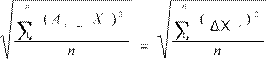 σ =
σ =
, (1.13)
where is the numerical result of an individual measurement, n is a number
measurements.
The nature of the curves described by (1.13) is shown in fig. 1.4, and for three values of σ. The function (1.4) is graphically represented by a bell-shaped curve, symmetric with respect to the ordinates, asymptotically
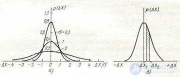
Figure 1.4
approaching the x-axis. The maximum of this curve is obtained at
 ΔX = 0, and the value of this maximum is p (ΔX) max = l / σ 2π. As can be seen from fig. 1.4, the smaller the σ, the narrower the curve and, consequently, the more rarely large deviations occur, i.e., the more accurately the measurements are made.

As noted earlier, the arithmetic average of the measurement series A is only the most reliable value of the measured value. It is of interest to determine the error in calculating the arithmetic mean value. This error is estimated using values similar to those by which the error of an individual measurement is estimated. If we perform k series of measurements, in each of which n separate measurements are made, and calculate the arithmetic average value for each series, then the obtained average

 the arithmetic values of А 1, А 2, А 3, ..., А n will differ slightly among themselves. These average values will differ from the true value X of the measured value by random variables and, therefore, will be distributed around X according to Gaussian law (1.4). To get an idea of the random variation of the arithmetic mean with respect to the exact value X of the measured quantity, it is necessary to calculate the standard deviation of the mean from the arithmetic mean. In the theory of errors, it is proved that this deviation is n times smaller than the mean square error of an individual measurement, i.e.

 , (1.14)
σ A - mean square error of the mean
Where
arithmetic from a series of measurements; σ is the standard error of a single measurement; n is the number of measurements in the series. From this expression it is seen that increasing the number of repeated measurements of n leads to a decrease
σ A measurement result. mean square error
In practice (especially with a small value of n), it is necessary to evaluate the accuracy and reliability of the results obtained for the mean value and the mean square deviation. For this purpose, use the confidence level and the confidence interval. By confidence probability we understand the probability of an error occurring that does not exceed some accepted boundaries. This interval is called the confidence interval, and the probability characterizing it is called the confidence probability.
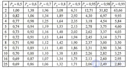
In practice, it is necessary to estimate the errors according to the results of a relatively small number of measurements. The use of formula (1.14) in this case gives an underestimated value of the confidence interval, i.e., the estimate of the measurement accuracy is unjustifiably too high. In this case, the confidence interval can be refined using Student's coefficients tn, which depend on the given confidence probability p and the number of measurements n.
To determine the confidence interval, the mean square error must be multiplied by the student coefficient. The final result can be written as:
 A = A ± t n σ A , (1.15)
The values of the coefficients tn required in the calculations are given in Table. 1.1.
General information about the processing of measurement results
Table 1.1 Student coefficients t (Pd, n)
1. List the possible causes of errors.
2. Name the signs by which errors are classified.
3. What is called absolute, relative and reduced errors?
4. What are gross errors (blunders)?
5. What error characteristics do you know?
6. Formulate the properties of the systematic, random and progressive components of the measurement error.
7. Give examples of methodical errors known to you.
8. What are the methods to reduce systematic errors?
9. When can the measurement error be considered as a random variable?
10. What are the basic laws of the distribution of random errors.
11. How is Student Distribution described and used?
12. What is called confidence level and confidence interval?
13. Name the rules for rounding measurement results.
14. List the algorithms for processing the results of direct multiple measurements.
15. Tell us about the three sigma criteria.

Comments
To leave a comment
METROLOGY AND ELECTROradio-measurement
Terms: METROLOGY AND ELECTROradio-measurement