Lecture
Below is considered one of the possible options for implementing the command transfer algorithm. Its main features:
Thus, the algorithm implements the most difficult case and, in a specific application, can be simplified if one of the listed conditions is abandoned. For example, in modern stations with distributed control, control groups can be so reduced that they can be managed without reserve and repetition if a command is not executed.
The block diagram of the command transfer algorithm is shown in Fig. 3.5.
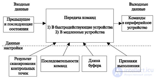
On the structural diagram, as in the previous case (scanning algorithm), the input information (previous and subsequent states) is shown. As we have already mentioned, the sequence of commands that is to be transmitted is searched for with this information. In addition, the input of the algorithm receives information from the scanning algorithm - the result of scanning control points; This information is used to validate the transmission of commands.
The remaining information is entered before the start of the algorithm and is the setting information.
A sequence of commands represents a table that associates a sequence of commands with each pair of states.
Signs of execution are recorded in each command and indicate the method of command execution (consistent, by condition, by time).
The buffer length is calculated based on the load on the module, and indicates the maximum number of applications that may be in the queue for the execution of the command transfer algorithm.
The algorithm is presented in fig. 3.6. He begins work when he receives an application for the transfer of a sequence of commands (operator 1). This application contains two states (previous and next). Sometimes these pairs are numbered, and then information about the number of the pair, called the sequence number of the command, is transmitted. This information is used to select a sequence of commands (operator two) corresponding to this input information. Next, put the current number of the first command of the sequence (operator 3), followed by the formation of the current command (operator 4). The formation consists in the fact that according to the number of the device type, which is contained in the first command, read from the sequence table, the set number is substituted from the process area of the connection manager. Further, this command is transferred to the buffer for output with the "waiting for transfer" sign.
When a command is output, the presence of this sign is checked - operator 5 (other signs are possible, for example, “waiting for control”).
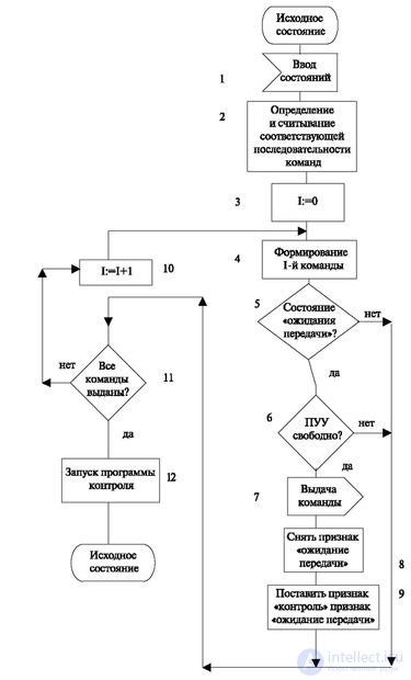
Operator 6 checks the i-PU free. When you turn on slow peripherals, it can be busy and it makes sense to go on to transfer the next command, if it is sent to another PUU.
The operator transmits commands, after which the "waiting for transmission" is removed, the "control" feature is set, and when all commands are transmitted, the second part of this algorithm is activated - "control over command transmission" (operators 8-9).
Then the need to further transfer at least one more command (operator 11) is checked, and if necessary, the command counter is incremented by one (operator 10). In the case of the transfer of the last command, the control algorithm is started (operator 12). Next, the algorithm goes to its original state.
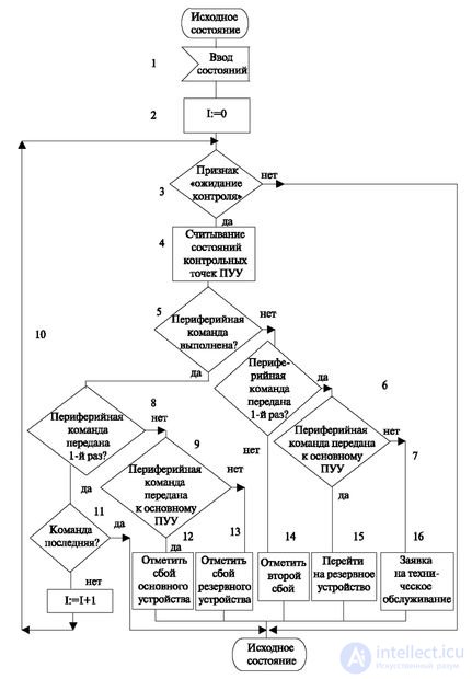
Let us now consider the second stage of issuing commands - control of the issuance (Fig. 3.7) The algorithm shows that the transfer of commands is initiated by the central program, and upon detection of requests, begins the execution of control. It checks if the given command sequence has the feature "waiting for control". If there is such a sign, then it is checked whether the command is executed or not. If it is done, it is determined whether it happened the first time or not; then it turns out what device it was done - the main or backup. In accordance with the results of the verification of these conditions, the actions displayed in the operators that do not require explanations are carried out. At the end of the usual checks are done at the end of the transfer.
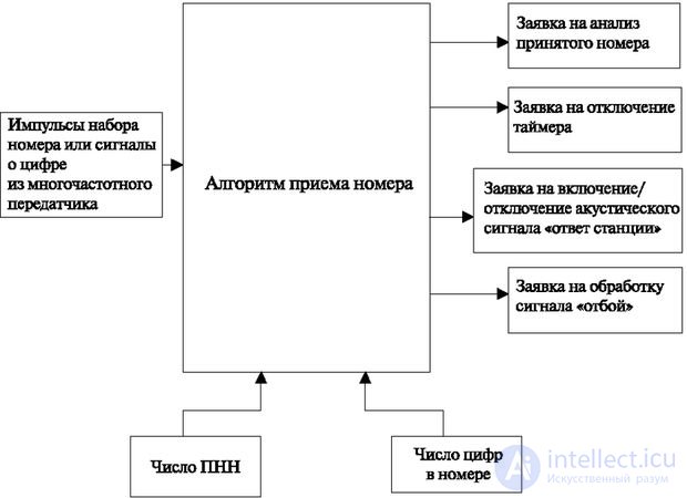
The algorithm is designed to fix the number of the called subscriber.
It should be able to receive a number from a disk and multi-frequency dialer. From the point of view of the maintenance process, these two types of dialing differ in that the information comes in either as separate pulses (disk dialing) or directly as a digit code.
The algorithm for receiving the number provides:
Output data (results) are (see fig. 3.8):
The algorithm uses the following memory areas:
A specific example of the algorithm is shown in Fig. 3.9.
The operation of the algorithm begins with an analysis of the buffer of requests (operator 2).
If there are no bids, control is returned to the dispatcher algorithm.
If there are job applications, then:
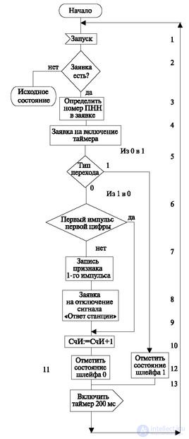
Often time is counted by the number reception algorithm itself. For this, control is transferred to this algorithm every 100 ms. If the loop is open, that is, the state has changed from 1 to 0 (operator 5), then the number of the incoming pulse is analyzed (operator 6). If this is the first pulse, then a request is generated to turn off the station response signal (operator 8) and it is noted that the first pulse of the first digit is received (operator 7).
The contents of the counter is increased by 1 (operator 9). If the pulse is not the first, then the same operator 9 is performed, and the above actions are not carried out. Then the state of the loop is fixed to 0 (operator 11), and the application is read again. If the type of transition from 0 to 1, then the loop state is fixed to 1 (operator 11), the 200 ms timer is turned on and the buffer request is read again.
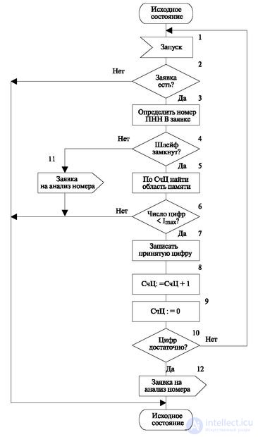
The second part of the number reception algorithm (Fig. 3.10) begins with an analysis of the presence of requests for a timer (operator 1). If there are no applications, the algorithm finishes the work. If there are requests, the algorithm determines the number of the dialing receiver (operator 2) and the state of the loop is analyzed. In the case of a closed loop, the operation of the algorithm depends on the number of digits recorded by the SC counter (operator 5). If the number of digits exceeds the specified maximum value (operator 6), the algorithm ends the work. Otherwise, the digit fixed in the pulse counter is rewritten into the corresponding memory area (operator 7), and the counter value (digit) is increased by 1 (operator 8). The pulse counter is reset (operator 9), after which it is analyzed whether there are enough numbers accumulated to start the establishment of the connection (operator 10). In the case of a positive result, a request is generated for the number analysis algorithm (operator 12). If there are no applications for the algorithm (operator 2), then a request is generated for the "hang up" signal processing algorithm (operator 11).
Interaction with the central program consists in recording incoming numbers in the memory of this program. In addition, the module can work separately, but most often it sets the state when receiving a number as part of the process states and makes an application for scanning dialing receivers from the same name.

Comments
To leave a comment
Telecommunication Services and Devices
Terms: Telecommunication Services and Devices