3: 1 Algorithms of individual functions performed in program-controlled stations

Annotation: In this section, only one of the algorithmic support levels is considered. In accordance with the recommendations of the CCITT (Z.100 series "Specification and Description Language SDL"), the stages of software development are outlined. In this case, two types of algorithms are defined: algorithms for the specification stage and algorithms for the description stage

The specifications show the station’s work from the customer’s point of view and are written using the customer’s terminology. For example, they include algorithms for incoming communication, outgoing and others, describing the operation of the station from the point of view of the highest level. The following is the development of algorithms that implement these functions.

In this course we will talk about part of the description stage algorithms. For a more detailed consideration of the development of algorithmic software can be found [6], [9]. Below in this lecture will be used the terms and symbols that are set out in the CCITT recommendations. Below are some of them.

The algorithm is depicted as a model of a finite automaton [9]. The following terms are used to describe its operation:

• INPUT - a signal coming from the external environment;
• OUTPUT - the signal transmitted by the algorithm to the external environment;
• STATUS - position of the algorithm at which the process is suspended until an INPUT signal is received;
• TRANSITION - a set of actions that, when an ENTRY signal arrives, transfer an automaton from one state to another;

These actions, besides the EXIT signal, contain:

• SOLUTION - choosing one of several possible ways to continue the process;
• TASK - an action that is neither a DECISION nor an OUTPUT.

For these operators, graphic symbols are used to describe their image ([9], [16]).

Typically, description-level functions are specification of specification level symbols. Some algorithms for these operators are discussed below.

For example, the scanning algorithm, which is given first in this lecture, gives a description of the implementation of the INPUT operator at the specification level. The algorithm for receiving the number gives a description of the implementation of one of the tasks of the specification level, etc.

Note that these functions were considered in the previous sections when it came to station control devices of the coordinate system in another implementation.

General provisions

All functions of control devices implemented in hardware can be implemented by programs. Therefore, in the 1980s, all stations basically switched to software control. Each hardware device can be associated with a software module.

Consider the algorithms for performing some of the most massive modules. We will pursue two main goals:

1. Outline the algorithms of the main modules involved in establishing the connection.
2. Using examples of specific, fairly common module algorithms, demonstrate the possibilities of generalization.

In our reasoning, we will proceed from the general model of the algorithm shown in Fig. 3.1.

Fig. 3.1. Structural diagram of the station operation algorithm

To build a general algorithm of this type, we assume the presence of replaceable modules that implement individual functions and are caused by a central program. In this case, the modules themselves must meet special requirements.

First, they must have an external interface and be used, as well as a microcircuit, as necessary. Unlike most microcircuits, the module can be configured (currently, many microchips have this property). Adjustment can be carried out by quantitative indicators or a choice of modes.

It is assumed that, having a base module and initial data, it is possible to obtain (generate) a specific module. Naturally, the program module is usually accompanied by the text of the control problem for its verification (the latter will not be considered in this lecture).

Thus, an algorithmic module is a replaceable unit capable of tuning to a given mode or equipment.

The basis of the mathematical model is an automaton principle.

Each of the modules will be displayed as a virtual machine that controls specific equipment or updates specific memory areas. In doing so, it will have virtual inputs and outputs.

Inputs are divided into two groups: operational and configuration inputs. The formalization of the modules of the algorithms in the form of logical formulas will be presented below.

The brevity of our presentation in this section is based on the principle of "less details", therefore, following the key line of research, the algorithms will be presented in general terms.

Scanning algorithm

So, we have established that the software can be implemented on the basis of a universal program. The first part of such a system is an input algorithm. Consider one of the most common input algorithms - scanning, i.e. input by periodic polling.

Some features of the scanning algorithm are generated by the structure of the equipment.

Sensors to be scanned to determine call arrival (hereinafter, we will call them “scan points”) are included in the scan “rulers”. They form matrices called determinants. A station can have several identifiers - from 1 to 100. Therefore, the address of each scan point is determined by the number of the identifier, the number of the ruler in the determinant, and the number of the point in this ruler. In fig. 3.2 shows these inputs, which give the software the necessary parameters. Some of the points can be blocked, for which a table of locks is set up that contains “masks” that exclude some points from the scanning process. The number of determinants, the number of rulers, the blocking table, the number of points in the ruler refer to semi-permanent data representing equipment parameters.

In addition, there are semi-permanent data related to the process.

Due to the nature of the service process, the following data must be entered relating to the process:

1. The number and value of scan periods (usually the value of the period duration is indicated in the number of 10 ms intervals).
2. Scanning schedule, i.e. a table assigning period values ​​to individual rulers.
3. Scan table, where the addresses of scanned lines are located. They are located in rows in the table and are divided into lists. Each list contains addresses of scanned lines arranged in the order of their polling. For example, the first is the list of lines polled every 10 ms, then the list of lines polled every 20 ms, and so on.
4. The length of the ticket buffer. This parameter sets the buffer length for storing the received applications for call processing programs. It is set after a probabilistic calculation of the number of incoming calls.

In fig. 3.2 shows the operational inputs and outputs:

1. Signal generator signal. It sets the beginning of the process of polling the next line. As we already mentioned, in most systems the minimum period is 10 ms.
2. Request to scan to the specified address. This application comes from the operator or program, if any rulers are not scanned periodically or an extraordinary check of their condition is required.

The signal "response word" is also shown as an input signal. This is a response to the polling line signal. Its appearance depends on the scan mode.

enlarge image
Fig. 3.2. General view of the scanning algorithm

In fig. 3.2 also indicates the modes in which the scanning algorithm can work:

1. A simple scan, which consists in the fact that during periodic polling the status of the ruler is read (encoded 1 - there is a change in the polling point and 0 - there is no change). The state of all points of the ruler is fed back to the input of the scan module as an n - bit word (n is the width of the ruler and is usually 16 or 32).
2. Mode with protection. Scanned sensors are usually in contact with the external environment (subscriber and connecting lines, relay contacts) - this causes the appearance of short-term interference. To combat this phenomenon is applied scanning with protection. The most common method is a double (triple) scan with a comparison of the results. For further processing, only signals that are stable are transmitted, i.e., they persist longer than a predetermined time.
3. Scan by checkbox. In many cases, the input signal comes in the event of the end of the accumulation of data. For example, when a caller's number is received from a neighboring station, the numbers accumulate at the incoming station and a connection request is generated after a sufficient number of digits have been received. In such cases, only one sensor (flag) is scanned, which is an indicator of receiving a signal that the information has been received. After the flag is triggered, all information is read.
4. Another type of scan - on request. This is a scan when an application for scanning is recorded from outside (from an operator or program).

In accordance with the scanning mode, the application is formed. In fig. 3.2 shows the types of applications.

In fig. 3.2b shows the application for a simple scan.

It contains the address of the scanned ruler:

• type of identifier - indicates the devices included in this determinant (many of them contain several scan points);
• the number of the determinant is the number of the determinant in the type;
• the line number is the number inside the determinant.

In fig. 3.2b shows the information requesting scanning by request. It contains the address of the scanned ruler and the address of the process (memory area) to which the result should be written.

In fig. 3.2g shows the structure of the response word. In this case, information is provided for simple scanning and scanning with protection and on request. It contains the applicant's number, i.e., the program or equipment that has submitted the application for scanning. Further information about the scan point is presented in the coordinates of the equipment, that is, the type of set (AK, ISBK, etc.) and the number of the set among the type Point number - the number among the point of scanning among this set. Next comes information about the type of change. In most cases, it is shown that the interviewed point has changed its state — namely, it has moved from a state denoted by zero (the initial state) to a state denoted by one (the working state). Sometimes, a scanning program is required as a result to specify one of two transitions — for example, from the initial state to the working state and vice versa. Then, taking into account the need to display the absence of a change, two bits are provided for the "type of change" field. They indicate: 00 - no change, 01 - change from the initial state to the working state and 10 - change from the working state to the initial state.

When scanning for the checkbox in the field "type of change" indicates all received information, the completion of the reception of which signaled the checkbox.

The information obtained during the scanning process is the source for the selection and activation of further programs.

Fig. 3.3. Principles for the distribution of applications for different organization of the schedule

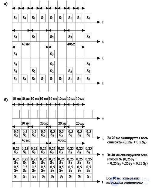
When the scanning algorithm works, the organization of scanning address lists plays an important role (Fig. 3.3a). In memory, scan address lists are grouped on a period basis. For example, suppose that the same S ₁ list contains the addresses of the lines scanned with a period of 10 ms, the list of S ₂ includes the addresses of the lines scanned every 20 ms, and in S ₃ all the lines scanned with a period of 40 ms. Suppose that in the first period all lists are polled, then after 10 ms only lists S _{1 with a} period of 10 ms are polled (for the other lists — S ₂ and S ₃ — the scan did not expire). In the second cycle, lists S ₁ and S ₂ will be polled. Then only one list S ₁ will be scanned again. Next - all three lists. As a result, the number of scanned addresses will change - then decrease, then increase, - which can lead to a congestion of requests in separate 10-millisecond cycles (see the resulting graph in Fig. 3.3a).

Therefore, a slightly different procedure for polling lists is adopted (Fig. 3.3b). In this case, the addresses of the lists are divided into parts, the number of which is equal to the number of 10-millisecond cycles that make up the period. So, for example, the S ₂ list (scan period of 20 ms) is divided into 2 parts, the S ₃ list is divided into four parts (scan period of 40 ms).

In addition, every 10-millisecond cycle scans the entire list of S ₁ , half (0.5) - S ₂ , a quarter (0.25) - S3. This ensures in each period an equalization of the number of scanned lines (see the resulting graph in Fig. 3.3b) and ensures a high probability of a uniform receipt of applications in different 10-millisecond cycles.

Communication with the central algorithm is as follows:

1. when working with an existing process, the scan results (in the formats shown in Fig. 3.3d) are recorded in the corresponding process memory area specified in the application; together with the state of the process they are the initial data for the transition;
2. during the initial call, an application for opening the process memory is written, then the input signal is written to it and the new process is placed at the end of the processing queue. This setup allows you not to delay the processing of existing calls and is one of the measures to combat processor overload during peak loads.

After processing the central algorithm, a scanning application is written in the memory area of ​​the algorithms, where the object from which the INPUT signal is expected and the number (address) of the process area where the application is to be installed is indicated.