Lecture
We will consider linear stationary dynamical systems described on the time interval [0 , t f ), where t f > 0, by the differential equation [M1] with the initial conditions t (0) = 0,  ,
,  , ...,
  and sufficiently smooth input action u ( t ).
2 .2.1. Transients. The solution of the differential equation [M1] is the function
(2.18)  ,
,
which at t = 0 satisfies the initial conditions, and for any  equation [M1]. The concept of phase variables of the system, to which the functions,
  ,
,  , ...,
  ( t ), satisfying the equation [M1], and the concept of a transient. The transition process is the process of change in time of various system variables (phase and input variables, deviations, etc.), during which the system changes its state. The transition process can be obtained in an analytical or graphical form. The graphic forms of the transition process include
, , ..., u ( t ), etc .;
Fig. 2.3. Transients: timing charts and phase trajectory
Decision can be represented as
(2.19) 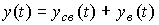 ,
,
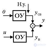
those. contains two components. Forced component  (t) corresponds to the transition process of the system [M1] under the initial conditions:
  and is the response of the system to the input action u ( t ). Free component
  (t), or the transition process of an autonomous system, corresponds to the solutions of a homogeneous differential equation [M1 a] and depends on the initial conditions
  ,
,  , ...,
2.2.2. Autonomous system processes. The behavior of the autonomous system and the free component of the transition process ( t ) depends on the poles of the system, i.e. the roots  characteristic equation
  (see also clause 3.3). Roots take real values
 ,
,
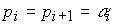
or represented by complex conjugated pairs:
 ,
,
where α i = Re p i is the real part of the root,  - the coefficient of the imaginary part.
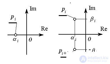
Fig. 2.4. System poles
For the case of unequal roots, the free component is determined by the expression:
(2.20) 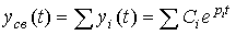 ,
,
Where 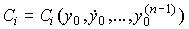 - undefined coefficients,
  - free oscillations of the system, or mode .
Real root  corresponds to the aperiodic component of the transition process
(2.21) 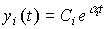 ,
,
Fig. 2.5. Aperiodic process
A pair of complex-conjugate roots of the characteristic equation corresponds to the vibrational component
(2.22) 
 ,
,
Where  - amplitude
  - phase of oscillation
  i is the angular frequency.
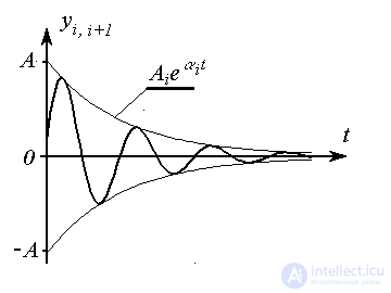
Fig. 2.6. Oscillatory process
If among the roots of the characteristic equation are equal, then the expression (2.20) is not valid. So, a pair of equal real roots
corresponds to the aperiodic component of the transition process
(2.23)  .
.
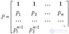
To find the particular solution y St ( t ) corresponding to the given values of the initial conditions , , ..., and the values of C i in the formula (2.20) use the method of undefined coefficients [1]. In accordance with the method from formula (2.20), it is necessary to obtain general expressions for phase variables.  , , ..., and for t = 0 write n algebraic equations
(2.24) 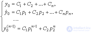
The equations contain n unknowns С i , which are found by one of the known methods. For example, you can rewrite equation (2.24) in a vector-matrix form
 ,
,
Where 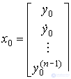 ,
,  ,
, 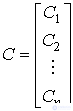 .
.
and find the column vector of unknown coefficients as
 .
.
If for some values of the initial conditions the identity
= y *,  ,
,
where y * = const, then the value y = y * is called the equilibrium value of the output variable (or equilibrium position) of the autonomous system [M1a]. In the equilibrium position can be written
(2.25) = y *, , ...,  .
.
After substitution (2.25) in the equation [M1a] we find
(2.26) a n y * = 0.
Provided that a n & nequal; 0 , we find that the only equilibrium position of the system under consideration is the origin
(2.27) y * = 0,
and for a n = 0 we find an infinite set of equilibrium values.
Remark 2 . 1 . Provided that the real part  some real or complex root p i is strictly negative, i.e.
(2.28)  ,
,
the corresponding component of the transition process eventually fades:
 .
.
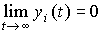
If condition (2.28) holds for all  , the whole free component is damped:
(2.29)  ,
,
moreover, the limit value of the output variable exactly coincides with the equilibrium position of the autonomous system y * = 0 .
2.2.3. Forced movement. The transient component of the transient depends on the input action and can be analytically determined only for a number of special cases corresponding to some typical input signals. The most common signals are single jump,  -function and harmonic input.
Consider the response of the system to a single step function (a single jump)
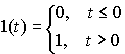 ,
,
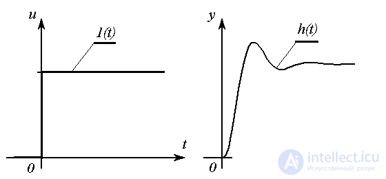
Fig. 2.7. Single race and transition function
Forced component  solutions
  when acting on the system [M1] input of a single step function
  is called a transition function (characteristic) of the system, i.e.
(2.30) 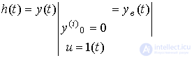
Consider the response of the system to a single impulse function (delta function) ( t ). The latter is defined as
(2.31) 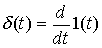
or an impulse of infinitely large amplitude A and infinitely small duration  satisfying the condition
(2.32)  .
.
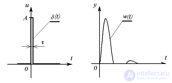
Fig. 2.8. Delta function and weight function
Forced component  solutions when a pulse function is applied to the system [M1] input
  is called the weight function (characteristic) of the system, i.e.
(2.33) 
Note that, given the definition (2.33), it is easy to get
(2.34)  .
.
For arbitrary input effects  the forced component of the transient process of the system [M1] can be found by the formula (convolution integral)
(2.35)  .
.
In the particular case when  (t), by virtue of property (2.34), we find
 .
.
Note that in the general case, finding the forced component of the transition process with the help of integral expressions of the type (2.35) (see also (2.42) in § 3.2.1) is difficult. A much simpler task is to find the established component of the transition process.
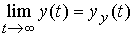
2.2.4. Steady movement. The motion of the system, considered for sufficiently large values of t (  ), is called steady state. Accordingly, the established component of the transition process
  called the forced component
  at
at  i.e.
i.e.
(2.36)  .
.
Function  is a particular solution of the equation [М1], obtained under certain (usually non-zero) initial conditions and depends on its right side, i.e. input effects .
Remark 2.2. Often, the following form of system solution representation [M1] is used:
(2.37)  ,
,
Where  - the transitive component, or the general solution of the equation [M1], which can be found in the form similar to (2.20), i.e.
(2.38)  ,
,
where C i ' - constant coefficients.
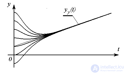
Fig. 2.9. Transients and steady state
Provided that for all values of p i ,  (see Remark 2.2), the free component of x St (as well as
  ) decays, i.e. the expression (2.29) holds. Then
(2.39)  ,
,
those. the steady state corresponds to the transition process of the system in steady state. On the other hand, if one of the modes of the system y i ( t ), and hence the free component as a whole, increases indefinitely, then the limit (2.39) does not exist, and the concept of the steady state loses its meaning.
Typical particular solutions of the linear equation [M1], corresponding to the steady-state components of the transition process when acting on the system of typical input signals u ( t ), are found by the known rules:
| u (t) | y y (t) |
| U 0 | Y 0 |
| U 0 + U 1 t | Y 0 + Y 1 t |
U 0 sin  0 t 0 t |
Ysin ( 0 t +  ) ) |
where U 0 , U 1 , Y 0 , Y 1 , ; 0 , - permanent.
2.2.5. Static mode The most important special case of the system [M1] solution corresponds to the constant input action  and the established component
(2.40)  .
.
Let the free component of the system decay, i.e. property (2.39) holds and, therefore,
 .
.
The last formula shows that for sufficiently large t (  ) there is no movement in the system, i.e. There is a static mode of operation.

The solution of equation (2.39) in the static mode is sought in the form
(2.41)  ,
,
Where  - undefined coefficient. Considering the fact that
  write down
(2.42) 
 ,
,
and from equation (2.41) we find that
(2.43)  ,
,  .
.
After substituting (2.41) - (2.43) in [М1], we obtain a simple algebraic expression
(2.44)  .
.
Let be  . Then the indefinite coefficient K is found as
(2.45)  .
.
With  will get
  where (see clause 2.1)
  i.e. в этом случае ( 2.44 ) не является частным решением уравнения [M1].
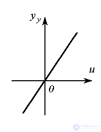
Зависимость установившейся составляющей (выходной переменной после окончания переходного процесса)  от величины входного сигнала
  =const называется статической характеристикой динамической системы. Для линейных систем вида [M1] статическая характеристика представлена уравнением прямой (2.41), где постоянная
  , рассчитываемая по формуле (2.45), называется коэффициентом передачи или статическим коэффициентом системы.
Система [M1], для которой  и следовательно существует статическая характеристика называется статической системой.
Астатической называется система, для которой  и следовательно, не существует статической характеристики, а установившийся режим невозможен.
Определение статической характеристики сводится к элементарной операции нахождению статического коэффициента K 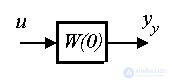 по формуле (2.45), где a n и b m - соответствующие коэффициенты дифференциального уравнения [М1]. Однако статическая характеристика может быть получена и из операторной формы [М2] или [M3]. Сопоставляя (2.45) и [ М3 ] , найдем
(2.46)  .
.
Следовательно, в статическом режиме система описывается уравнением
(2.47)  .
.
Замечание 2.3. По аналогии с определением положения равновесия автономной системы, можно ввести понятие равновесия возмущенной системы (2.40) при постоянном входном воздействии i.e. положения, в котором выполняется тождество
 = y *,
and therefore
(2.48) = y *, , ...,  .
.
Нетрудно показать, что равновесное значение выходной переменной y* в точности совпадает с установившимся значением, т.е.
(2.49) 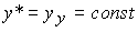 .
.
В частном случае при u=0 получаем автономную систему [M1а] и равновесное положение  .
.

Comments
To leave a comment
Mathematical foundations of the theory of automatic control
Terms: Mathematical foundations of the theory of automatic control