Lecture
As noted in § 3.1.1, various ways are possible to select state variables of a dynamic system. The ambiguity of this choice determines the non-uniqueness of the input-state-output models [M4], [M5] (or [M6], [M7]) corresponding to a particular input-state model [M1] ([M2] or [M3]), since the choice of other state variables leads to a different model of BCB. On the other hand, the original model of BCB can be specially transformed, which is usually associated with changes in the basis (system of coordinates) of the state space  . This kind of transformation is called equivalent, or similarity transformation .
3.4.1. Equivalent conversion . Let the input-output model of a single-channel system (control object) be given by the operator equation
(3.93) a ( p ) y ( t ) = b ( p ) u ( t ),
Where
 .
.
and  - the roots of the characteristic equation (system poles), or the equation [M3], where
(3.94)  ,
,
and the model ENE is obtained in the form [М6], [М7]. We introduce a new (transformed) state vector:
(3.95)  ,
,
Where  - transformation matrix (similarity), satisfying the condition
  . Then there is an inverse transformation
(3.96)  .
.
Differentiating (3.95) and substituting (3.96), [М6] we find:
(3.97) 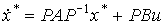
and
(3.98)  .
.
The resulting expressions are rewritten as
[M6 * ] 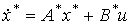 ,
,
[M7 * ]  ,
,
Where
(3.99) 
(matrix like A ),
(3.100)  ,
,
(3.101)  .
.
Such matrices have the following properties:
but) 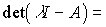

b) 

The model [М6 * ], [М7 * ] is called the equivalent (similar) model [М6], [М7]. Fairly obvious property:
(3.102) 
 ,
,
those. for such systems, the connections of the output and input variables are preserved, and, therefore, the BB [M1], [M2], [M3] models.
3.4.2. Canonical representations of models VSV . The simplest input-state-output models corresponding to the initial equations of the system [М6], [М7] are called canonical representations ( forms ) .
Diagonal shape is a model represented by the equations of state
(3.103) 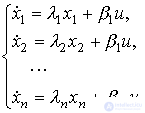
and the output equation
(3.104)  .
.
(Fig. 3.24). The model can be written in a compact form [M6 *] [M7 *], where
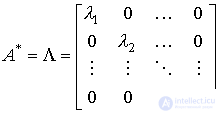 ,
, 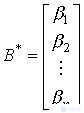 ,
, 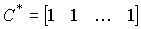 .
.
Systems with different poles are diagonalized. 
 . At the same time (see clause 3.1.3) of the matrix of the main and transformed system are related by
(3.105)  ,
,
those. transformation matrix is like
(3.106)  .
.
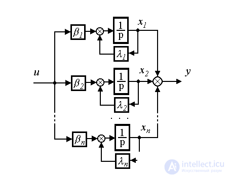
Fig. 3.24. The block diagram of the canonical (diagonal) form
The model of a fully controlled system [10] can be reduced to a controlled (Frobenius)) canonical form
(3.107) 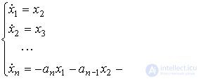
and
(3.108)  ,
,
(Fig. 3.25). This form corresponds to the vector-matrix equations [M6 *] [M7 *], in which

 ,
, 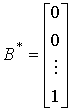 ,
,
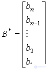
C * = [ b n b n -1 ... b 2 b 1 ] ,
 and
and  - the coefficients of equation (3.107),
a T = [ -a n - a n -1 ... -a 2 -a 1 ] , 0 = [0 0 ... 0 0] T ,
I is the unit matrix of size ( n- 1)  ( n- 1). State matrix
  is called the accompanying matrix of a polynomial
  or Frobenius matrix.

Fig. 3.25. Canonical controlled form
The transformation matrix to the canonical controllable form is as
(3.109) P = U * U -1 ,
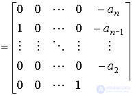
where U and U * are the controllability matrices of the initial [10] and canonical [10] models, respectively. For the case of n = 3, the following holds:
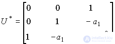 .
.
The model of a fully observable system (see [10]) can be reduced to the observable (Frobenius)) canonical form of the form :
(3.110) 
and
(3.111)  ;
;
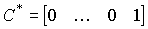
(Fig. 3.26). This canonical form corresponds to the vector-matrix equations [M6 *] [M7 *], where  - accompanying (Frobenius) matrix of the species

 ,
,  ,
,  ,
,
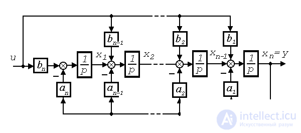
Fig. 3.26. Canonical observable form
The transformation matrix is as
(3.112) P = ( Q * ) -1 Q,
where Q and Q * are the observability matrices of the original and canonical models [10]. For the case of n = 3, the following holds:
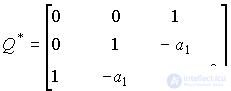 .
.

Comments
To leave a comment
Mathematical foundations of the theory of automatic control
Terms: Mathematical foundations of the theory of automatic control