1.5 Blocks and control algorithms

The control unit of the system designed to solve local problems, discussed in Section 1.4, includes the master unit (ST) and the output variable controller (Fig. 1.23).

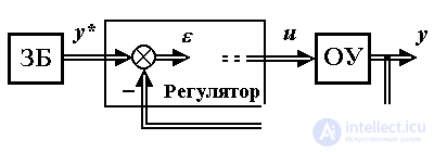
Fig. 1.23. Multichannel control system

Remark 1.8. In modern systems, a block does not necessarily correspond to a physical device, in most cases it is an algorithm or program for calculating the required variables (signals), which corresponds to the cybernetic interpretation of the block concept (see clause 1.1).

1.5.1. Regulators. A regulator is a block (algorithm) that calculates a control action u to solve a local control problem. A control algorithm is a set of analytical expressions used to calculate control actions (the term "algorithm" comes from the name of Al-Khorezmi and implies a system of operations carried out according to certain rules).

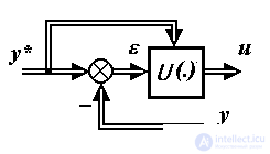
A typical control algorithm for the output variable y is:

(1.11) u = U ( , y *, ... ) ,

where is the mismatch calculated by the formula:

(1.12) = y * - y,

and algebraic and transcendental functions, as well as integro-differential operators, Laplace operators, Boolean functions, etc. can act as the operator U (·).

The simplest control algorithms (regulators) are regulators of the form deviation :

(1.13) u = U ( ).

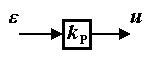
These include: proportional, or P-controller , for which

(1.14) u = k _P e ,

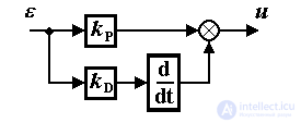
where k _P is a constant coefficient; proportional-differential, or PD-controller :

(1.15) ,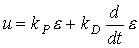

where k _D is a constant coefficient;

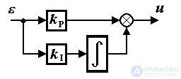
proportional-integral, or PI controller :

(1.16) ,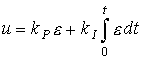

where k _I is a constant coefficient, as well as a proportional-integral-differential ( PID controller )

(1.17) .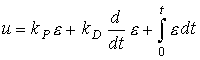

1.5.2. Master blocks The master unit is a block (algorithm) that performs the calculation of the driver action y * ( t ). In the simplest cases, master knobs and remote controls act as such blocks, and in more advanced systems, hardware and software implemented generating signal generators act.

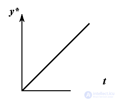
The simplest master blocks can be attributed to the blocks that generate signals for stabilization problems, where y * = Y * = const, and elementary tracking tasks. So for the organization of the movement of the control object with a constant speed = V * = const the algorithm described by the differential equation is used.

, y * (0) = Y *,

providing signal generation y * ( t ) = Y * + V * t. For motion with constant acceleration = const algorithm is applied

, y * (0) = Y *, ,

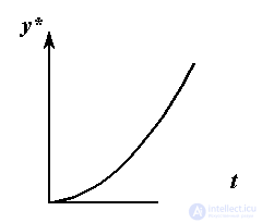
generating signal y * = Y * + V * t + a * t 2/2 , etc.

A more complex master unit is an interpolator - a multichannel master unit, designed to calculate the current values ​​of the agreed master effects (see clause 1.4), i.e. signals y _j * ( t ), subordinate to the functional dependence:

(1.18) ( y ₁ *, y ₂ *, ..., y _m * ) = 0.

The output signals of the interpolator are used in tracking systems that provide a solution to the problems of coordinated control and, in particular, the trajectory control of multi-link mechanical systems, where the desired trajectory of movement of the working point S of the mechanism is given by equation (1.8).

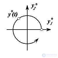
Example 1.7. The interpolator of the control system of a robotic arm, the gripper of which moves in a circle (1. 10), generates a two-dimensional driving force

y * ( t ) = {y ₁ * ( t ) , y ₂ * ( t ) }

and is described by a system of differential equations

(1.19)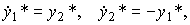

with initial values ​​of y * ₁₀ = R , y * ₂₀ = 0. The system has a solution

(1.20) y * ₁ = R cos t, y * ₂ = R sin t,

which satisfy equation (1.10).

Many modern self-propelled guns are built as object state management systems , i.e. provide solutions to stabilization problems

x = x * = const

or state tracking , i.e. compliance with a given law of change of the state vector:

x = x * ( t )

where x * = {x * _i } is the vector of defining influences by state. The control algorithms of such systems are

(1.21) u = U ( e, x *, ... ),

where the mismatch e is calculated by the formula:

(1.22) e = x * - x.

The structure of the state management system is illustrated in fig. 1.24.

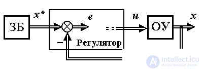
Fig. 1.24. Condition management system

1.5.3. Special units of control and monitoring systems. To solve the problems of automatic control arising both in ACS and in control systems, observers and identifiers are used.

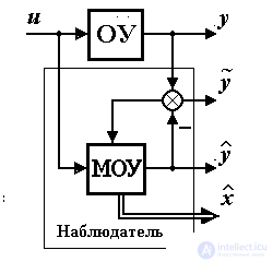
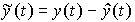
An observer is a block (algorithm) intended for estimating non-measurable state variables of the OS x _i or the external environment. The structure of the OU observer includes the model of the control object MOU, which produces the current values ​​of the assessment ( t ) output variable y ( t ) and estimates ( t ) state vector x ( t ). The behavior of the model is adjusted by feedbacks due to observation error ( discrepancy )

.

The observer is used in state control systems (Fig. 1.25), in which not all state variables can be measured or measurements x _i contain significant interference. In these cases, the control algorithm considered earlier (1.21) takes the form

(1.23) u = K ( , x *, ... ) ,

where is the mismatch score calculated by the formula:

(1.24) = x * - .

The mathematical model (equation) of the control object contains the coefficients _i - mass inertia, electrical and thermodynamic parameters of the controlled process and other devices used in ACS. Parameters are combined into a parameter vector.

= { _i }

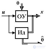
In cases where the values ​​of the parameters change over time or are not known in advance, it becomes necessary to use parameter identifiers. Identifier is a block (algorithm) of the form

(1.25) ,

Where (·) Is a dynamic operator intended for estimating the parameters of an OS, i.e. calculating in real time the current estimate value ( t ) vector According to the available information on the current state x ( t ) and the input effect u ( t ) of the object.

Identifiers are used in adaptive control systems , i.e. in systems in which the parameters of the controller are configured during system operation. They use adaptive control algorithms of the form:

(1.26) u = U ( e, x *, ... ) ,

where is the evaluation vector can be obtained using the identification algorithm (1.25).