3.3 Phase trajectories of an autonomous second order system

Consider a second-order autonomous system:

(3.74) ,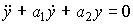

with initial values , . System characteristic equation

(3.75)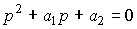

has two real or complex-conjugate roots (poles of the system):

(3.76) ,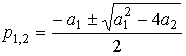

whose location on the complex plane determines the type of transient processes

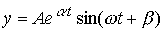
(3.77) y = y (y ₀ , , t )

and dynamic properties of the system (see § 1.4.1).

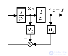
Define state variables as phase variables: , . The state-exit model takes the form:

(3.78) ,

(3.79) ,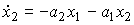

(3.80) ,

with initial values , Eigenvalues ​​of the system matrix

coincide with the roots of the characteristic polynomial (3.75) p _1,2 .

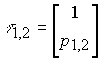
Own vectors _1.2 (see § 3.1.3) of the second-order system under consideration are found (provided that its poles are real) from the expression

,

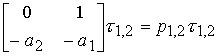those.

and the corresponding eigenspaces R _{1,2 are} represented by straight lines.

(3.81) x ₂ = p _1,2 x ₁ .

The equilibrium (steady) states ( x ₁ *, x ₂ * ) of the system (3.78), (3.79), (3.80) are found from the condition

(3.82) , .

When a ₂ 0 we find that the equilibrium position is the origin

(3.83) x ₁ * = 0 , x ₂ * = 0 ,

and for a ₂ = 0 we find the set of equilibrium states (straight line)

(3.84) x ₂ = 0.

Recall that the integral curve ( phase path) of the system under consideration is the hodograph of the state vector = when the parameter t changes , and the set of phase trajectories obtained for different initial conditions form its phase portrait (see § 3.1.2). Phase trajectories can be obtained experimentally or found analytically. In the latter case, use the following technique. Equations (3.78), (3.79) are written as

dx ₁ = x ₂ dt,

dx ₂ = - (a ₂ x ₁ + a ₁ x ₂ ) dt.

After dividing the second expression by the first, we obtain the differential equation

(3.85) .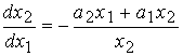

The solution of this equation is sought in the form

(3.86) x ₂ = _one   ( x ₁ )

and determines the integral (phase) trajectory of the considered

systems on the plane r ² .

Consider transients corresponding to different values ​​of the roots of the characteristic equation (poles of the system (3.78) - (3.80)).

1. For unequal real roots (Fig. 3.4, 3.5)

(3.87) p _1,2 = _1.2 =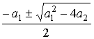

equation (3.74) has a solution

(3.88) ,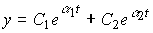

which corresponds to the aperiodic process (see § 2.2.2).

Provided that a ₁ > 0 and a ₂ > 0,

Re p _1,2 = _1.2 <0,

(Fig. 3.4). In this case, there is a damped transient, the condition

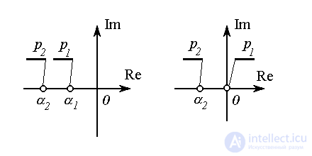
Fig. 3.4

Fig. 3.5

(3.89)

and phase trajectories of the system with t converge to the equilibrium position O (Fig. 3.6), which is called a stable node . (A system of this kind belongs to the class of asymptotic-stable systems [11,12]). The system has two proper (invariant) subspaces R ₁ and R ₂ , on which the solutions of equation (3.74) are written as

Fig. 3.6

Fig. 3.7

(3.90)

and

(3.91)                       ,

those. the dynamics on the eigenspaces corresponds to the behavior of the first order system.

Provided that a ₁ > 0 and a ₂ = 0, we get

Re p ₁ = <0, p ₂ = 0,

(Fig. 3.5). Phase trajectories of the system (Fig. & 3. 7) with t converge to the set of equilibrium states (straight line R ₀ ) described by equation (3.84). This set is its own subspace of the system. (A system of this kind belongs to the class of stable, or neutral-stable, systems, see [10,12])

Provided that a ₁ <0 and a ₂ > 0,

Re p ₁ = ₁ > 0, Re p ₂ = ₂ <0,

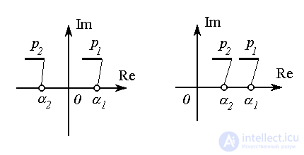
Fig. 3.8 Figure 3.9

(Fig. 3.8). In this case, there is a divergent transition process. Phase trajectories of the system with t diverge (Fig. 3.10):

(3.92)

with the exception of trajectories starting on the straight line R ₂ , for which the limit relation (3.89) is satisfied. (A system of this kind belongs to the class of unstable systems, see [10,12]) The equilibrium position of the system (point O ) is called a saddle point (saddle) . The system has two proper (invariant) subspaces R ₁ and R ₂ , on which the solutions (3.74) are written in the form (3.90) or (3.91).

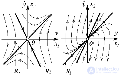
Fig. 3.10 Figure 3.11

Provided that a ₁ <0 and a ₂ <0,

Re p ₁ = ₁ > 0, Re p ₂ = ₂ > 0,

(Fig. 3.9). In this case, there is a diverging transition process and all phase trajectories (Fig. 3.11) of the system at t diverge (performed (3.92)). The equilibrium position of the system (point O ) is called an unstable node (and the system is also unstable). The system also has two proper (invariant) subspaces R ₁ and R ₂ .

2. If , then the system has equal real poles (fig. 3.12 - 3.14)

p _1,2 = =

and the solution of equation (3.74) takes the form:

Fig. 3.12 Figure 3.13 Figure 3.14

y = (C ₁ + C ₂ t) ,

corresponding to the aperiodic process (see § 2.2.2).

Provided that a ₂ > 0 (and a ₁ > 0),

Re p _1,2 = <0,

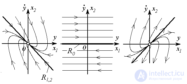
Fig. 3.15 Figure 3.16 Figure 3.17

(fig. 3.12). In this case, a decaying transient takes place, the limiting relation (3.89) is fulfilled, phase trajectories at t converge to the equilibrium position (stable node) O (Fig. 3.15) and the system is asymptotically stable. The eigenspaces of the systems R ₁ and R ₂ coincide.

Provided that a ₁ = a ₂ = 0, we get

p ₁ = p ₂ = 0,

(Fig. 3.13) and the divergent transition process. Phase trajectories of the system (Fig. 3.16) with t go to infinity, with the exception of trajectories starting at the set of equilibrium states (line R ₀ ), described by the equation x ₂ = const, and the system is unstable.

Provided that a ₂ <0 and a ₁ <0,

Re p _1,2 = > 0,

rice 3.12) ,. proper subspaces of the system coincide. In this case, the limiting relation (3.89) holds, phase trajectories at t diverge. The equilibrium position O is an unstable O node (Fig. 3.17) and the system is unstable.

3 If performed , then the system has complex conjugate poles (Fig. 3.18-3.20)

Fig. 3.18 Figure 3.19 Figure 3.20

and the solutions of equation (3.74) take the form

which corresponds to the oscillatory process (see § 2.2.2).

The system with complex poles considered here does not have its own subspaces.

Provided that a ₁ > 0 and a ₂ > 0,

Re p _1,2 = <0,

(fig. 3.18). In this case, there is a damped oscillatory transient process. Running (3.89), phase trajectories of the system at t converge to the equilibrium position O (Fig. 3.21), which is called a stable focus, and the system is asymptotically stable.

Provided that a ₂ = 0, Re p _1,2 = 0, the system has pure imaginary roots

p _1,2 = - j

(fig. 3.22) is also called a linear oscillator (see § 2.3). In this case, a continuous oscillation process takes place. The phase trajectories of the system are represented by closed concentric curves (elliptical orbits), and the system is (neutral) stable. The equilibrium position of the system (point O ) is called the center

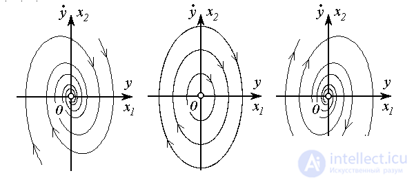
Fig. 3.21 Pic. 3.22 Figure 3.23

Provided that a ₁ <0 and a ₂ <0,

Re p _1,2 = > 0,

(fig. 3.20). In this case, there is a diverging oscillatory transition process. Phase trajectories of the system with t diverge from the equilibrium position O (Fig. 3.23), which is called an unstable focus , and the system is unstable.