4.2 Models of driver units and external influences

For the description of the external environment, the objects of tracking and generation of driving forces in program control systems, there is a need to design additional dynamic models ( external action generators ), the output of which is perturbing or specifying the y * ( t ) effect (see § 1.2.1). For smooth functions and y * ( t ) the corresponding disturbing and driving effects generators (driving blocks) can be obtained in the class of autonomous linear models similar to those previously considered [M1a], [M2a] or [M6a], [M7]

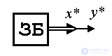
Thus, the master block of a BZ (generator of master actions) can be described by a homogeneous differential equation of the form

(4.24)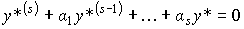

with constant coefficients _i and initial values

(4.25) , ,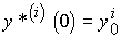

or corresponding vector-matrix equations of state

(4.26)

and exit

(4.27) ,

Where 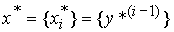- s - dimensional vector of tasks (generator state) with initial values ​​of coordinates .

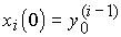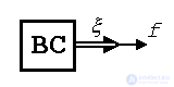
The generator of smooth disturbing influences (model of the external environment of the Armed Forces) is described by a homogeneous equation

(4.28)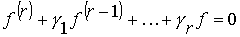

with constant coefficients _i   and initial values

(4.29) ,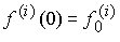

or in a compact form

(4.30)

(4.31)

Where 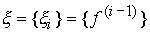- r - dimensional vector of the state of the environment with the initial values ​​of the coordinates .

The impacts generated by the considered models correspond to the solutions of differential equations (4.26), (4.27) and (4.30), (4.31), i.e. functions

(4.32)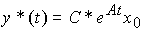

and

(4.33) ,

respectively. In particular cases, using such models can be obtained:

• polynomial effects

(4.34) ,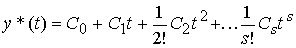

Where - constants, defined as

(4.35) ;

• harmonic effects

(4.36) ,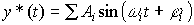

where a _i , _i and _i - constants, corresponding to amplitudes, phases and frequencies of harmonics, etc.

To build an impact model for a given function y * ( t ) (or ) you can use the method of sequential differentiation of the corresponding analytical expressions

(4.37) y = y * ( t )

(or f = f (t)), represented, for example, in the form (4.34) or (4.36).

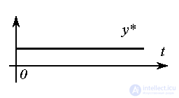
Example 4.1 . To obtain a model of a constant signal

(4.38) y * (t) = C ₀ ,

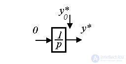
let's differentiate the last expression by time. Get the first order equation

(4.39)

with initial value y * (0) = С ₀ .

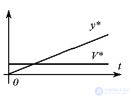
Model of linearly increasing signal (uniform motion)

(4.40) ,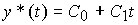

is obtained by a double differentiation. In the first step we get

(4.41) ,

and on the second - the desired differential equation

(4.42) .

To obtain the initial conditions from equation (4.40), we find y * ( 0 ) = С ₀ , and from equation (4.41) - * (0) = C ₁ .

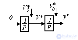
Equation (4.42) is reduced to the form of a state model (a system of equations in the form of Cauchy). To do this, in addition to the main state variable that coincides with the output variable y * ( t ), the second variable V * ( t ) (travel speed) is introduced:

(4.43)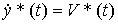

with initial value 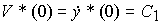. Equation (4.42) can be rewritten as

(4.44) .

The obtained equations (4.43) and (4.44) describe the desired model of the state of the master block.

Note that the solution of equation (4.42) or system (4.43), (4.44) (i.e., expression (4.40)) can be written as

(4.45) .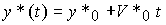

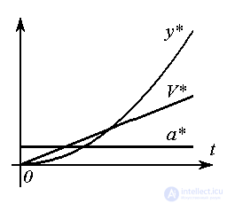
The model is quadratically increasing signal

(4.46)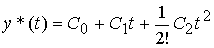

(uniformly accelerated motion) is obtained as a result of the procedure of three-fold differentiation of expression (4.46) and has the form

(4.47)

with initial conditions

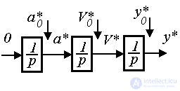
y * (0) = C ₀ , * (0) = C ₁ and . To build a state model of the considered master block, state variables y * ( t ) , V * ( t ) , a * (t) are introduced, where - acceleration, and after their differentiation in time and corresponding substitutions, a system of equations is obtained

(4.48) ,

(4.49) ,

(4.50)

with initial values ​​of y * (0) = C ₀ , V * (0) = C ₁ , a * (0) = C ₂ .

Note that the solution of equation (4.47) or system (4.48), (4.49) (i.e., expression (4.46)) can be written as

(5.51)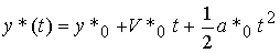

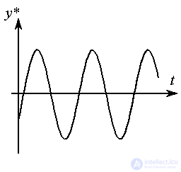
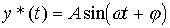
Example 4.2 . To generate the simplest harmonic effect

with frequency i.e. signal

,

the model of single-frequency linear oscillator is used (conservative, see p. 2.3):

(4.52) .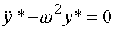

Amplitude amplitude A and phase shift determined by the initial values ​​of the model y (0) and .

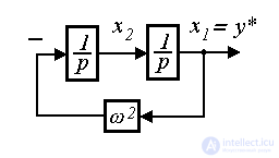
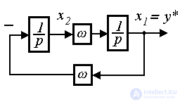
Model (4.52) is easily reduced to Cauchy form.

(4.53)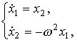

with exit

(4.54) .

Here the following notation is entered:

(4.55)

In the particular case to build a signal generator

(4.56)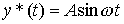

state variables are entered

(4.57)

(4.58)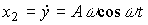

with initial values

(4.59) , .

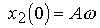After time differentiation of expressions (4.57), (4.58) and corresponding substitutions, we obtain the system of equations (4.53).

Remark 4.1. If state variables are selected as

(4.60) ,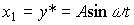

(4.61)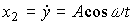

with initial values , , then the state model of the master oscillator takes the form

(4.62)

For generation of nonsmooth functions y * (t) and f (t) are used.

• nonlinear dynamic models [10];
• variable structure models [10];
• non-autonomous linear models of the form:

(4.63)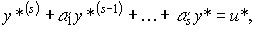

Where - non-smooth (may be discontinuous) input effect of the model.

Example 4.3. To generate a signal y * ( t ) with a trapezoidal velocity graph (Fig. 4.6) you can use the model:

(4.64)

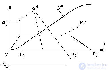
Fig. 4.6. Non-Smooth Signal Processes

or - in the form of Cauchy

(4.65) ,

(4.66) ,

where a * = a * ( t ) is the type acceleration signal

(4.67)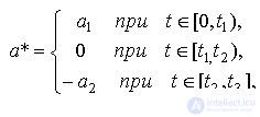

where a ₁ > 0 and a ₂ > 0 are constant.