Lecture
The state of a system is a set of such variables, the knowledge of which allows, with a known input and known equations of dynamics, to describe the future state of the system and the value of its output. The choice of state variables is ambiguous.
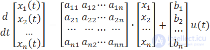
The state space method is fairly universal; it can be applied to nonlinear systems of multidimensional systems. For an initial introduction to this approach, linear one-dimensional systems (or SISO - Single Input Single Output) are considered below, the equations of which have the following general form:

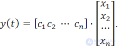
where X ( t ) is the state column vector [ n × 1]; And the matrix of the coefficients of the object [ n × n ]; B - entry matrix [ n × 1]; u ( t ) is the control signal; Y is the output vector [ k × 1]; C is the output matrix [1 × n ]; D is the matrix of the influence of an input directly on the output of the system [ n × 1] (it is often assumed that D = 0).
The equations of state of the SISO-system in expanded form:
The system described by matrices A and B is controllable if there is such an unbounded control u ( t ) that can transfer an object from the initial state X (0) to any other state X ( t ).
For a SISO system with one input and one output, the concept of a controllability matrix (size  ):
):
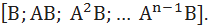
If the determinant of this matrix is non-zero, then the system is controllable.
Modal synthesis involves the formation of such feedbacks on the state in which a given location of the poles of a closed system is provided. Mode is the component of the solution of a differential equation corresponding to a particular pole .
The location of the poles mainly determines the nature of the transition process in the system. Such root assessments of the quality of the transition process, such as the time of the transition process, the degree of stability, oscillation and re-regulation are usually considered.
To assess the performance of the system uses the concept of degree of stability  which is understood as the absolute value of the real part of the root nearest to the imaginary axis (because the roots having the smallest real part in modulus give the most slowly decaying component in the transient process).

The stability margin of the system is estimated by oscillation. The system tends to oscillate if the characteristic equation contains complex roots. 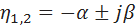 .
.
Oscillability is estimated by the formula

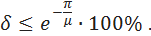
The value of the oscillation can be estimated overshoot
For an object defined by the equations of state (1), the state control is described by the expression
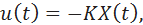
where K is the vector of feedback coefficients.
Thus, the system, closed regulator, is given to the following form:
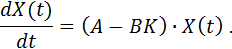
This expression corresponds to fig. 1, where g (t) is the driving force.
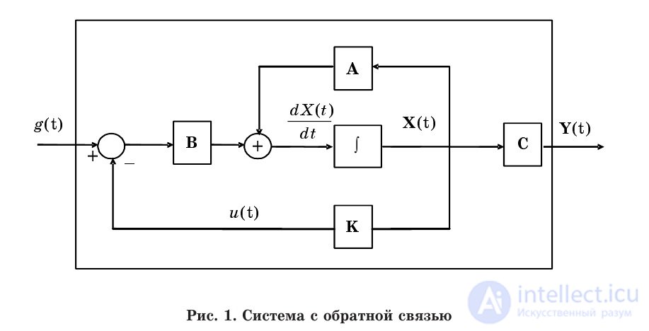
Fig. 6.1. Feedback system
Akkerman proposed a formula that would allow using a similarity transformation to translate a model of an arbitrary structure into a canonical form of controllability, determine the sought K coefficients and then recalculate the solution obtained as applied to the original structure. Ackerman’s formula is [3]

where B is the coefficients of the characteristic polynomial of the matrix ( A - BK ) .
Thus, the problem of modal synthesis is reduced to choosing the desired roots of the characteristic polynomial of a closed system, at which the specified parameters of the transient process are provided, after which, according to the standard algorithm, the feedback coefficients by state are calculated.
>> w1 = ss (A, B, C, D),
where A , B , C , D are matrices of the model.
From the model in the state space, you can get the PF command:
>> w2 = tf (w1)
And vice versa, if the model specified by the PF already exists, then it can be transformed into the state space using the ss command:
>> w = tf ([2 2], [3 4 1]);
>> w1 = ss (w)
We note that, in general, different models in the state space can correspond to the same TF, but the same TF corresponds to all these models.
The manageability matrix can be built using the ctrb function, which is called by one of the commands:
>> W = ctrb (A, B)
>> W = ctrb (sys)
>> W = ctrb (sys.A, sys.B)
In the MatLab package, there is acker function with which you can ensure the desired location of the poles of a one-dimensional linear system (in accordance with Ackermann formula):
>> k = acker (A, B, P),
Where A and B are the system matrices; P is the vector that specifies the desired location of the poles of the system.
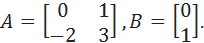
An example . Let the system be described by matrices.
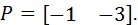
The desired poles are given by the vector:
Then you can calculate the value of feedback coefficients using the commands
>> A = [0 1;, 2 3];
>> B = [0; one];
>> P = [, 1, 3];
>> K = acker (A, B, P)
K = 1 7
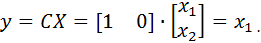
Thus, the control in this example should be in the form

For multidimensional systems, MatLab has a place function (it can also be used for one-dimensional systems). Function
>> K = place (A, B, P)
calculates the matrix of feedback coefficients K , which provides the desired location of the poles of the system. The length of the vector P must be equal to the number of rows of the matrix A.
 . For this calculation, we write the equations of state in the form:
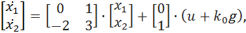
substituting equation (6), we have:

In the steady state we get
and the condition must be met

Therefore, from equation (7) we get

The input effect should be multiplied by this factor.
In the Simulink MatLab simulation package, there is a State Space block for describing an object in the state space. However, this block does not allow to directly evaluate the current value of the state vector, therefore, in order to simulate the modal controller operation, it is necessary to describe matrix operations in detail.

Comments
To leave a comment
Mathematical foundations of the theory of automatic control
Terms: Mathematical foundations of the theory of automatic control