Lecture
Resilience - the property of the system to return to its original state after any impact
A linear dynamical system is called stable if, after removing the disturbances at
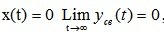 , that is, the motion fades (Fig. 6.1. a).
A system is called unstable if, after removing the disturbances, the free motion tends to к, that is, at t ??, 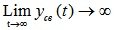 (Fig. 6.1. b).
A system is said to be neutral if, after removing the disturbances x (t), the free motion tends to some limit M , i.e. 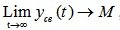 where 0 < M (Fig. 6.1. c).
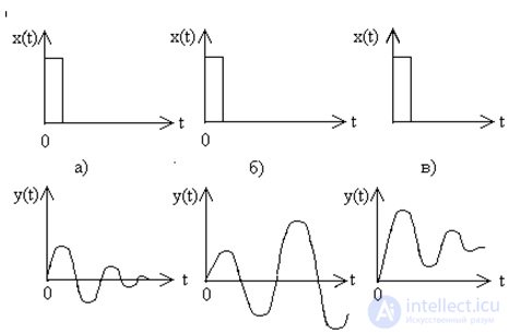
Fig.6.1. Free movement control system
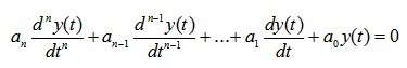
In the general case, the differential equation of a link or system has the form:
 (6.1)
(6.1)
His general decision
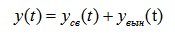 (6.2)
(6.2)
The component of the solution in the form of a general solution of a homogeneous equation is called the free movement y St (t) and the component in the form of a particular solution of the inhomogeneous equation is called the forced motion y exit (t), where y St (t) is defined by the left side of equation (6.1):
 (6.3)
(6.3)
His characteristic equation
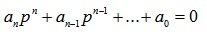 (6.4)
(6.4)
Since the concept of system stability includes only the fact of the presence or absence of attenuation of the transient process (regardless of the decay rate of the transient process), the stability of the linear system does not depend on the right side of the differential equation (6.1.) And is completely determined by its left side, i.e. (6.3 ).
The equation of motion of the system is represented by equation (6.1). For stability analysis, we investigate equation (6.3). His decision:
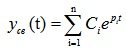
, where p i - roots of the characteristic equation (6.4).
Since, with an input effect limited in absolute value, the component of the forced motion is also limited, the stability of the system is ensured when the condition is met:
 (6.5)
(6.5)
which means that the transition process in the system fades.
Consider cases for roots of various types.
Real roots:
If all p i = ?, where? i is a really positive number, then

? i can have values> 0, <0, = 0.
From the properties of the exponential function we can conclude that when? i <0 and when t ??, the component y (t) is damped , that is, the system is stable.
Fig. 6.2. ? > 0 (system is unstable)
Fig. 6.3. ? = 0 (system on the verge of stability)
Fig. 6.4. ? <0 (system is stable)
Complex-conjugate roots:
I.e 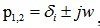 In this case, the solution component has the form:
 (6.6)
(6.6)
Where is A i ,? i , –constants defined by C i , C i + 1 ,.
Graphs of y i versus value? i are shown in Fig.6.5 and 6.6
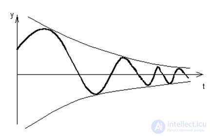
Fig. 6.5. Free movement of the system for the case of complex roots with negative real part
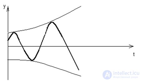
Fig. 6.6. Free movement of the system for the case of complex roots with a positive real part.
When ? i = 0, the roots are purely imaginary and the graph of the function is a continuous harmonic oscillations.
From the analysis performed, it follows that a linear dynamic system will be stable if and only if the real part of the roots of the characteristic equation is negative. This is a necessary and sufficient condition for the stability of a linear control system.
It should be noted that no real control system is strictly linear. Linear characteristics of links and linear differential equations are obtained by linearizing the real characteristics and equations.
Lyapunov proved that if the linearized system is stable, then the real system with small deviations is also stable; if the linearized system is unstable, then the real system is also unstable; if the linearized system is neutral or is on the oscillatory boundary of stability, then it is difficult to judge the stability of the real system, since small nonlinear terms can fundamentally change the type of transition process, making the system stable or unstable.
The disadvantage of the direct method of studying the stability of the system is the need to calculate the roots of the characteristic equation, which is associated with certain difficulties.
There are sustainability criteria that allow, without solving the equation, to answer the question: is the control system stable or unstable.
One of the most common algebraic stability criteria is the Routh-Hurwitz stability criterion , which was developed at the end of the 19th century. It is based on the analysis of the coefficients of the characteristic polynomial and reduces to checking the satisfaction of n inequalities (n is the order of the characteristic polynomial). The procedure for testing the stability of the AU by this criterion is as follows. From the coefficients of the characteristic polynomial  believing that
  compiled the main determinant of Hurwitz.
The system is stable if the Hurwitz determinant and all lower order determinants are greater than 0
Determinant Hurwitz
 (6.7)
(6.7)
From the main determinant of Hurwitz, the Hurwitz determinants of the lowest order (minors) are distinguished.
 (6.8)
(6.8)
The number of the Hurwitz determinant corresponds to its dimension.
The Routh-Hurwitz criterion is formulated as follows : for the linear automatic control system to be stable, it is necessary and sufficient that with all the Hurwitz determinants be positive, i.e.

For the linear system of equations to be stable, it is necessary and sufficient that the diagonal minors of the Hurwitz matrix are positive under the condition a 0 > 0. It can be shown that for equations of the first and second orders the condition of stability, according to Hurwitz, is the positiveness of their coefficients.
As with the use of the Hurwitz criterion, the initial information for using the Mikhailov criterion is the characteristic equation of the system under study. Here we apply a geometric illustration of the trajectory of the end of the Mikhailov vector - the Mikhailov hodograph.
On the basis of the characteristic equation of the closed system (6.4), we introduce into consideration a certain function of a complex variable, obtained by replacing p = j ?:
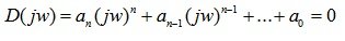 (6.9)
(6.9)
Function (6.9) can be represented as
 (6.10)
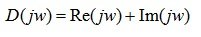
On the Re-Im complex plane, D (j?) Will describe the vector as it changes? from 0 to? curve - Mikhailov hodograph.
For a stable control system of the nth order, it is necessary and sufficient that the Mikhailov locus change when? from 0 to,, starting with the real positive semiaxis, passed counterclockwise successively through n - quadrants.
Figure 6.7 shows the Mikhailov locograph for various cases.
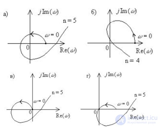
Fig. 6.7. Examples for the cases: a) stable, b) unstable systems, c) the case of a neutral system with a zero root, d) the case of an oscillatory stability boundary.
Refer to Figure 6.8, which illustrates a stable automatic control system. For a stable system of automatic regulation, the alternation of the roots of the actual Re (?) And imaginary jIm (?) Parts is observed (a consequence of the Mikhailov criterion).

Fig. 6.8. The change in the real and imaginary components of the Mikhailov vector with a change in frequency
The disadvantage of algebraic criteria and frequency stability criterion is their boundedness by systems without transport delay. In the case of a system with a transport delay, their application gives an approximate estimate of stability within the limits of the validity of the approximation of the link of transport delay next to Pade.
In 1932, the American scientist G.Naykvist showed that there is a definite connection between the stability and the type of AFCh amplifiers with negative feedback, and in 1936 the Soviet scientist A.V. Mikhailov extended the proposed criterion to automatic control systems. Frequency criterion of stability of Nyquist –Mikhailov, which allows to judge about the stability of a closed automatic control system by its amplitude - frequency characteristic in the open state. Since the latter can be obtained experimentally, this criterion is widely used.
An AC that is unstable in the open state may be stable in the closed state. This becomes apparent after analyzing the Nyquist-Mikhailov criterion.
This criterion makes it possible to judge the stability of a closed system from the AFC of an open system.
For minimum phase systems, this criterion is formulated as follows : for an automatic system, stable or neutral in the open state, to be stable in the closed state, it is necessary and sufficient that the AFCh curve of the open system does not cover the point M {-1, j0} on the complex plane when changing frequency? from zero to infinity and rotation of the AFCh vector W (j?) clockwise.
Fig. 6.9. An example of an unstable closed system with a stable open system (1) and the position of the system on the stability boundary (2)
Stability and stability margin
In Figure 6.10. the amplitude-phase characteristic of an open-loop system is shown  and a circle with a radius of R = 1.

Fig. 6.10. To the definition of the stability margin modulo and phase
The stability margin modulo is determined by the size of the segment AB. It shows how much you need to increase the amplitude of the amplitude-phase characteristics of an open-loop system.  without changing the phase so that the closed system reaches the stability limit:
 (6.11)
The stability margin of the phase is determined by the value
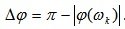 (6.12)
It shows how much clockwise it is necessary to rotate the phase without changing the amplitude of the amplitude-phase characteristic vector of the open-loop system so that the closed-loop system reaches the stability limit.
The stability of a closed SAR using a logarithmic criterion can be determined by constructing the combined LAFC and LFCH of an open-loop system.
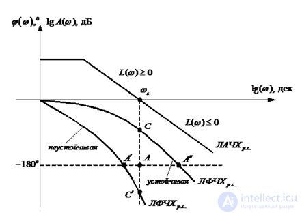
Fig. 6.11. System stability for LAFC and LPCHH
A closed automatic control system is stable if, at L (w)? 0, the corresponding LFCh passes in such a way that the phase? (W) does not exceed the value of -180 ° (-?).
The system stable in the open state will be stable and in the closed state, if the point A LFCh determined by the phase -180 ° (-?) Corresponds to the area of negative values of the logarithmic amplitude L (w);
An important indicator of the performance of the AU are the stability reserves in amplitude and phase.
The stability margin in phase is determined as the possible value of the increment of LFH until the stability limit is reached: ?? 3 =? +? (Wsr).
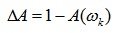
The stability margin in amplitude is determined as the possible value of the LAFH increment (i.e., the gain), at which the AC retains the stability L 3 = 20 lgR (w?) |.
Example 1. The transfer function of the system has the form:
 .
.
Check the system for stability. Investigate the stability of the system using the Hurwitz criterion.
Decision:
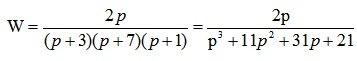
The characteristic equation of the system has the form:
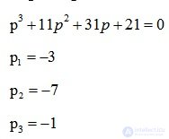
A necessary condition for the stability of the automatic control system: all the roots of the characteristic equation must be left (located in the second or third quarters of the coordinate plane). In this case, the necessary condition is satisfied.
Investigation of system stability using the Hurwitz criterion:
Let's make determinants of Hurwitz:
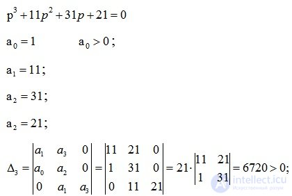
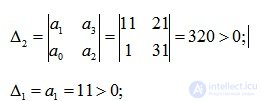
All Hurwitz determinants are greater than zero, hence the system is stable.
Example 2. Determine the stability of the system presented in Fig. 6.12 using the Nyquist and Mikhailov criteria.
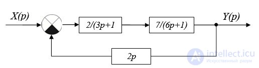
Fig. 6.12. Structural scheme
Decision:
Find the roots of the characteristic equation 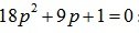 :
:
p 1 = -1 / 6;
p 2 = -1 / 3;
Both roots lie on the left side of the imaginary axis, which means that the open-loop system is stable.
Nyquist criterion:
Build AFCh open-loop system (Fig. 6.13).
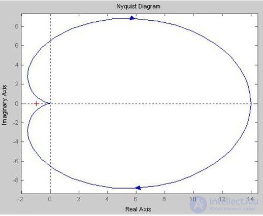
Fig. 6.13. AFC
Conclusion: for a closed system to be stable, it is necessary and sufficient that the AFC of an open system, when changing w from zero to infinity, does not encompass a point with coordinates (-1; j 0). In fig. 6.13 that the system does not cover the point (-1; j 0), it means that the system is stable.
Mikhailov's criterion:
We take the characteristic equation of the system:
On the complex plane, the graph of the imaginary part (Im) from the real (Re) vector H (jw) will describe as w changes from 0 to? curve - Mikhailov hodograph (Fig. 6.14).
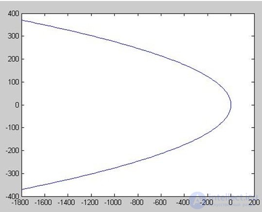
Fig. 6.14. Godograf Mikhailov
Conclusion:
In order for a closed system to be stable, it is necessary and sufficient that when w changes from 0 to? vector Mikhailov D ( jw ) turned to the corner  .
.
The resulting graph corresponds to the steady state of the system (Fig. 6.7), since when w changes from 0 to? vector Mikhailova turned to the corner . In this case, n = 2 (the order of the characteristic equation).
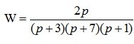
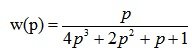
Example 3. Oscillatory link with the transfer function

covered by negative feedback through the integrating element (Fig. 6.15). Determine the stability of the system using the Nyquist and Mikhailov criteria under the following conditions:

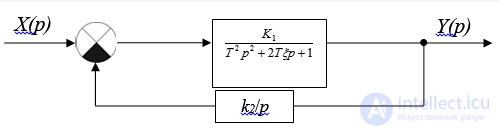
Fig. 6.15. Structural scheme
Decision:
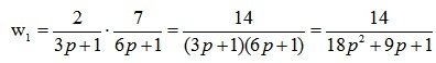
The transfer function of the system:
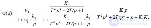
Substitute the values from the condition of the problem, we get:
Nyquist criterion:
We take the transfer function of an open-loop system, build an AFC diagram (Fig. 6.16).
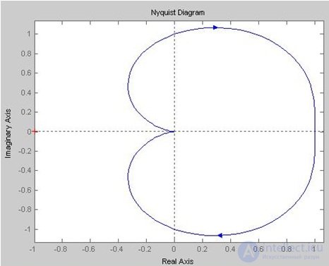
Fig. 6.16. AFC
Conclusion: for a closed system to be stable, it is necessary and sufficient that the AFC of an open system, when changing w from zero to infinity, does not encompass a point with coordinates (-1; j 0). In fig. 6.16 shows that the system does not cover the point (-1; j 0), which means the system is stable.
Mikhailov's criterion:
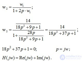
We write the characteristic equation of the system:
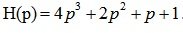
We introduce the function of a complex variable, replacing p with p = j ?. We get:
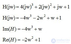
On the complex plane, the graph of the imaginary part (Im) from the real (Re) vector H (jw) will describe as w changes from 0 to? curve - Mikhailov hodograph (Fig. 6.17).
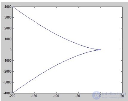
Fig. 6.17. Godograf Mikhailov
Conclusion: in order for a closed system to be stable, it is necessary to t enough so that when w changes from 0 to? vector Mikhailov D ( jw ) turned to the corner  .
.
The resulting graph corresponds to the unstable state of the system (Fig. 6.7).

Comments
To leave a comment
Mathematical foundations of the theory of automatic control
Terms: Mathematical foundations of the theory of automatic control