Lecture
A typical electromechanical object (EMO) contains a multichannel executive electric drive (EP, see § 1.2.1) and a controlled kinematic mechanism (KM). The multi-axis mechanisms of machine tools, robots, production lines, steering gears of aircraft and vehicles, moving parts of automatic equipment and instruments act as kinematic mechanisms of electromechanical systems. The drive serves to convert low-power electrical signals from a control device (control computer) into mechanical effects (forces and moments) of sufficient power applied to the load, i.e. to the kinematic mechanism. Each drive channel (see Fig. 4.1) provides the translational or rotational motion of the corresponding CM link and contains an input signal power amplifier (U), an electric motor (ED) and a gearbox.
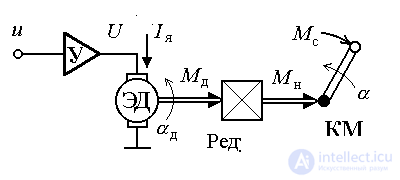
Fig. 4.1. Electromechanical object
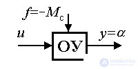
Consider a mathematical model of a single-channel electromechanical object (Fig. 4.1), which includes one rotational link of the mechanism and a single-channel electric drive. The output of the object is the angular displacement KM y =  , and its input is the control signal u ; the moment of resistance M c , applied to the load shaft, acts as a disturbing influence: f = - M c .
4.1.1. The exact model of EMO . To build a mathematical model of an object, equations known from physics that describe its functional elements are used.
The kinematic mechanism is described by equations derived from Newton's second law:
(4.1)  ,
,
(4.2) 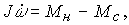
Where  - the speed of rotation of the shaft KM,
  - torque applied to the shaft,
  - reduced moment of resistance, J - reduced moment of inertia.
In the block diagram (Fig. 4.2), the mechanism is represented by two integrating links and a proportional link with a factor of 1 / J.
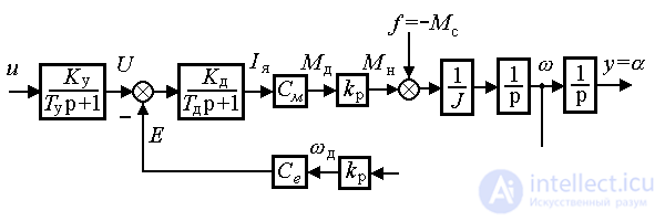
Fig. 4.2. EMO block diagram
The gearbox provides conversion (usually gain) of the motor torque M d at the load moment M n according to the formula
(4.3)  ,
,
where k p - the gear ratio of the gearbox ( k p = 1 / i p , where i p - the gear ratio of the gearbox). In this case, the speed of rotation of the ED d and shaft KM related by
(4.4) = k p .
In the block diagram, the gearbox is represented by proportional links.
The motor model is set by the torque characteristic
(4.5)  ,
,
where I i - the armature current, C M - mechanical constant, and the equation of the armature circuit
(4.6)  ,
,
where U is the voltage applied to the armature ED (power amplifier output), E is the counter-EMF, L and R are the inductance and resistance of the armature circuit, respectively. The last expression is convenient to bring to mind
(4.7)  ,
,
where T d = L / R is the time constant, and K d = 1 / L is the transfer coefficient of the anchor chain. Back EMF is determined by the well-known formula
(4.8) E = C e d = C e k p ,
where C e is the electric constant.
In the block diagram, the electric motor is represented as an aperiodic link (4.7) and two proportional links with transmission coefficients С e and С m .
The power amplifier is an aperiodic link, described by the equation
(4.9)  ,
,
where T y and K y are the time constant and the gain, respectively.
4.1.2. Building models of explosives and tertiary . Using the methods of transformation of structural schemes (see Section 2.4), using equations (4.1) - (4.9), the connection of the output of the object y = and its inputs u and f = - M c , i.e. EMO input-output model of the form [M2]:
(4.10) ( p 4 + a 1 p 3 + a 2 p 2 + a 3 p ) y ( t ) = b 0 u + ( d 0 p 2 + d 1 p + d 2 ) f ,
where a 1 , a 2 , a 3 , b 0 , d 0 , d 1 , d 2 are constant coefficients. Model (4.10) is reduced to the form [M3]:
(4.11) 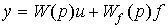 ,
,
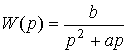
where W ( p ) and W f ( p ) are the transfer functions for control action and disturbance, defined by the expressions
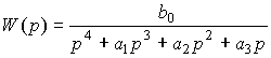 ,
, 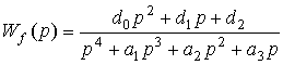 .
.
The input-state-output (VSV) model is constructed either on the basis of the model (4.10), or directly using the previously obtained equations of the functional elements of the object and the diagram in Fig. 4.2. In the latter case, equations (4.1) - (4.9) are converted to a system of 4 differential equations (Cauchy form) of the form:
(4.12) ,
(4.13) 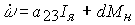 ,
,
(4.14)  ,
,
(4.15) 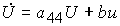 ,
,
where a ij , b, d are constant coefficients. The state vector is defined as
(4.16) 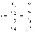 ,
,
and the disturbing effect - f = - M c . After this, the equations of state (4.12) - (4.15) are written in vector-matrix form
[M6f] 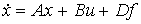 ,
,
and the output equation is obtained from the expression y = x 1 and is written in vector-matrix form
[M7]  .
.
Transient processes of the system with a single input action u = 1 ( t ) (state variables and the input action itself) are presented in Fig. 4.3.

Fig. 4.3. Transients of an electromechanical object
4.2.3. Approximate model of EMO . For the case when the inertia of electrical processes in the electric motor and power amplifier is not significant compared with the inertia of mechanical processes, the corresponding time constants T y and T d can be neglected. Putting T y = T d = 0 we rewrite equations (4.7), (4.9) in the form
(4.17) I = Kd ( UE ),
(4.18) U = K at u.
Then the equation (4.2) after substitution of expressions (4.3), (4.5), (4.6), (4.17) and (4.18) takes the form
(4.19) 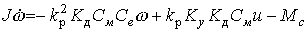
or
(4.20) 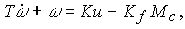
where T, K, K f - constant coefficients.
Thus, the approximate model of EMO is described by equations (4.1), (4.20) and is represented by integrating, aperiodic, and two proportional links (Fig.4.4). The input-output model is described by an operator equation of the form
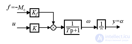
Fig. 4.4. The scheme of the approximate model of EMO
(4.21) ( p 2 + ap ) y ( t ) = bu + df ,
where a = 1 / T, b = K / T, d = K f / T are constant coefficients, and is reduced to the form (4.11), where
 ,
, 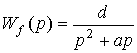 .
.
To obtain a model of VSV is determined by the state vector
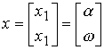 ,
,
and equations (4.1), (4.20) are rewritten as
(4.22)  ,
,
(4.23) 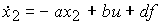 ,
,
Further, the system of equations (4.22), (4.23), as well as the expression y = x 1, are rewritten in the matrix form [М6f], [M7].
Transients for a simplified model of EMO with a single input action u = 1 ( t ) are presented in Fig. 4.5.
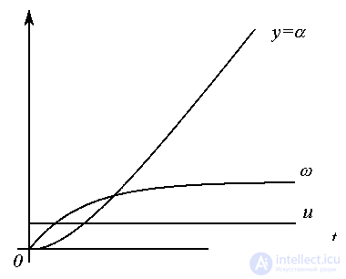
Fig. 4.5. Transients of the approximate model of EMO

Comments
To leave a comment
Mathematical foundations of the theory of automatic control
Terms: Mathematical foundations of the theory of automatic control