2.1 Linear input-output models

The mathematical model of a dynamic system is called the set of mathematical symbols that uniquely determine the development of processes in the system, i.e. her movement. At the same time, depending on the symbols used, analytical and graphic-analytical models are distinguished. Analytical models are constructed with the help of alphabetic characters, while grapho-analytical ones allow the use of graphic symbols (see clause 2.1.2).

Depending on the type of signals, continuous and discrete models of systems differ. Depending on the operators used - linear and nonlinear , as well as time and frequency models. Temporary are models in which the argument is (continuous or discrete) time. These are differential and difference equations written explicitly or in operator form. Frequency models involve the use of operators whose argument is the frequency of the corresponding signal, i.e. Laplace, Fourier, etc. operators

This section discusses continuous linear temporal models of dynamic systems.

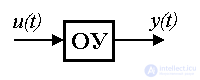
An input-output (BB) model is a description of the relationship between the input and output signals of a dynamic system. The need for such a description appears when considering the behavior of individual units and, in particular, the control object (OU), and the control system as a whole. Differences in the mathematical description of the blocks and the control system are not fundamental, but they require the use of different designations (see Clause 1.5). So, the input signal of the ACS is the specifying effect y * ( t ),   and the output is the variable y ( t ) . When describing blocks, the notation x ₂ ( t ) and x ₁ ( t ) are often used , respectively. In the following, we use the notation typical of the control object, where the input signal is the control action u ( t ) and the output is the variable variable y ( t ).

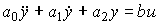
2.1.1. Analytical models. The linear input-output model of a single-channel dynamic system (here, the control object) can be represented by an ordinary differential equation of the form:

[M1] ,

where a _i , b _{i are} coefficients ( model parameters ), a ₀ 0   , b ₀ 0, n - model order, 0 m <n . Equation [M1] connects the input signals and their derivatives with output signals y ( t ) and their derivatives on some time interval, i.e. at . Meanings , , ..., are called initial values ​​(conditions ), and the number r = n - m 1 - relative degree of the model.

There are stationary systems for which the parameter values ​​are unchanged: , and you can put , and non-stationary models , where the parameters are functions of time, i.e. , . In the case when , the equation is called reduced.

System for which , called autonomous . The description of an autonomous system is given by a homogeneous differential equation of the form

[M1a] .

Model [M1] can be rewritten in operator form. To do this, we introduce into consideration the differentiation operators

and suppose that

.

Taking into account the introduced notation, the equation [M1] is easily converted to the operator form

[M2] ,

where differential operators are used

(2.1) ,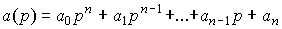

(2.2) .

The operator a ( p ) is the characteristic polynomial of the differential equation [M1], and the complex numbers , which are the roots of the characteristic equation

(2.3) ,

are called the poles of the system [M1] . The differential operator b (p) is the characteristic polynomial of the right side. Roots of the equation

(2.4) ,

those. complex numbers are called system zeros [M1].

From equation [M2] we find an explicit connection of the variables y ( t ) and u ( t ) in the form of an operator equation:

[M3] ,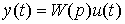

where is integral differential operator

(2.5)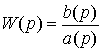

called the transfer function of the system [M1].

The advantage of using operator models like [M2] and [M3] is, firstly, the brevity of the corresponding equations, and secondly, the convenience of converting complex (composite) models (see Section 2.4).

Consider a special case of a dynamic system with coefficients b ₀ = b ₁ = ... = b _m-1 = 0 . When b _m = b 0 the system has a relative degree r = n-1 , and zeros are missing. The equation [M1] takes the form

(2.6) ,

equation [M2] -

(2.7) ,

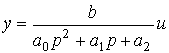
and the equation [M3] is

(2.8) .

Example 2.1. Let be and . The differential equation of the system has the form

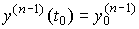
with initial conditions ; . Here - speed output variable. The operator form of the model is

,

and

.

System characteristic equation

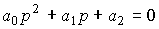
has two (real or complex) roots

.

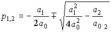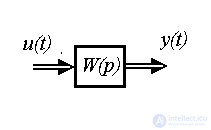
2.1.2. Structural schemes. The most common graph-analytical form of a dynamic system model is a structural diagram - a type of directional graph. Elements of such a scheme are (Fig. 2.1)

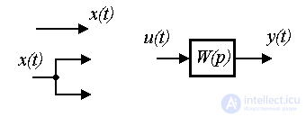
Fig. 2.1. Elements of the structural scheme

• letter designations of signals ( x ( t ) , u ( t ) , y ( t )   and so on) and so on;
• letter symbols of operators (for example, W ( p ));
• graphic symbols - arrows indicating the direction of the signals, nodes (signal forks), blocks with indication of the input and output signals, as well as operators describing the connections between the signals.

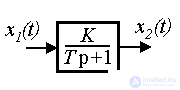
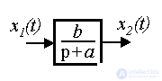
The simplest blocks used in structural schemes are (Fig. 2.2):

• unit of comparison;
• adder;
• proportional block;
• integrator

(see also clause 2.3).

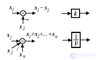
Fig.2.2. Simplest blocks

Example 2.2. The input-output heating furnace, RC-chains and motor acceleration (see Example 1 .1) are described by a first-order differential equation.

(2.9)

where T, K are constant coefficients (parameters). The operator form of the model is

(2.10) .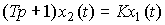

Here - the characteristic equation, which has one root (pole of the system) p ₁ = - 1 / T. From equation (2.10) we find the operator connection of the input and output

.

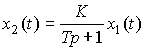
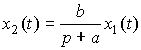
Therefore, the transfer function of the block is the operator

.

Note that equation (2.9) can be reduced to

(2.11)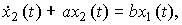

where a = 1 / T, b = K / T. Then the operator form (2.10) takes the form

(2.12)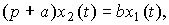

and form (2.12) is

.

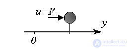
Example 2.3. Consider the motion of a material point of mass m under the action of a force (input action) u = F ( t ). This dynamic system is described by a second-order equation (Newton's 2nd law)

(2.13)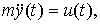

with initial conditions y ₀ = y ₀ (0), where y ( t ) is a linear displacement. The operator form of the model takes the form

(2.14)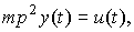

and the characteristic equation of the system

(2.15)

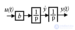
has two roots (poles of the system) p _1,2 = 0 . From equation (2.14) we find the operator connection of the input and output

(2.16)

where b = 1 / m . Therefore, the transfer function of the block is the operator

(2.17) .

In structural diagrams of multidimensional and multichannel systems, vector signals , and sometimes emit double arrows.

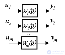
2.1.3. Multichannel models. First, we consider a multichannel system with independent (autonomous) channels. The system is described by m operator equations.

[M2m]

each of which characterizes the behavior of one of its channels.

Let us consider the vectors of output variables y and control u :

, ,

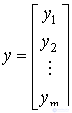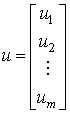accordingly, and we write the system of equations in vector-matrix form:

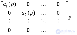
or,

[M2m] A ( p ) y = B ( p ) u

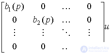
If matrix A ( p )   - is reversible, i.e. there is an inverse matrix

,

then from the equation [М2m] we find

[M3m] y = W ( p ) u,

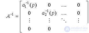
where W ( p ) = { W _ij } is the transfer matrix of the system (matrix integro-differential operator), calculated as

W ( p ) = A ^-1 ( p ) B ( p ) = .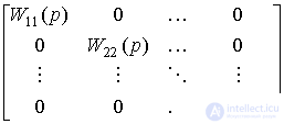

It is easy to see that in the considered case the transfer matrix is ​​diagonal, i.e.

W ( p) = diag { W _ii (p) } = { b _i (p) / a _i (p) }.

Now consider a multiply connected system , i.e. multichannel system with connected channels, described by a system of operator equations

a ₁₁ (p) y ₁ + a ₁₂ (p) y ₂ + ... + a _1m (p) y _m = b ₁₁ (p) u ₁ + b ₁₂ (p) u ₂ + ... + b _1m (p) u _m

a ₂₁ (p) y ₁ + a ₂₂ (p) y ₂ + ... + a _2m (p) y _m = b ₂₁ (p) u ₁ + b ₂₂ (p) u ₂ + ... + b _2m (p) u _m

[M2m] . . .

a _m1 (p) y ₁ + a _m2 (p) y ₂ + ... + a _mm (p) y _m = b _m1 (p) u ₁ + b _m2 (p) u ₂ + ... + b _mm (p) u _m

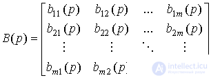
The system is reduced to the vector-matrix form [M2m], where

;

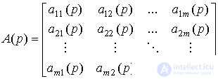and the form [M3m], where the transfer matrix W ( p ) is determined by the expression

W ( p ) = A ^-1 ( p ) B ( p ) =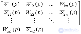

Model [M3m] can also be written in scalar form:

y ₁ = W ₁₁ (p) u ₁ + W ₁₂ (p) u ₂ + ... + W _1m (p) u _m

y ₂ = W ₂₁ (p) u ₁ + W ₂₂ (p) u ₂ + ... + W _2m (p) u _m

. . .

y _m = W _m1 (p) u ₁ + W _m2 (p) u ₂ + ... + W _mm (p) u _m

Note that the diagonal operators W _ii ( p ) belong to the main channels , and the remaining transfer functions W _ij ( p ) characterize the cross-links of the multichannel system.

For a two-channel multiply-connected system ( m = 2), we obtain:

y ₁ = W ₁₁ (p) u ₁ + W ₁₂ (p) u ₂ ,

y ₂ = W ₂₁ (p) u ₁ + W ₂₂ (p) u ₂ ,

where W ₁₁ ( p ) , W ₂₂ ( p ) are the transfer functions of the main channels of the system, and W ₁₂ ( p ) , W ₂₁ ( p )   - transfer functions of cross-links.

2.1.4. Perturbed model of the system. The disturbing effect f ( t ), which characterizes the effect on the control object of the external environment (see § 1.2), is considered as an additional input signal. 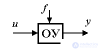Then the linear model of the single-channel dynamic system takes the form

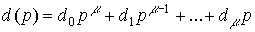
[M1f]

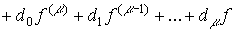
where d _{i are the} coefficients that determine the influence on the processes in the perturbation system f ( t ) and its derivatives f ^{( i )} ( t ) , d ₀ 0   , 0 <n . After substituting the differentiation operators p ⁱ and the corresponding transformations, we obtain the operator form of the model [M1f]:

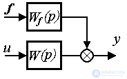
[M2f] ,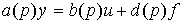

where differential operator is used

.

The explicit operator form takes the form

[M3f] ,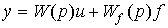

Where

.

the transfer function of the disturbing effects f ( t ).