4.3 Principles of control, models of regulators and closed systems

Recall that the control system consists of two main blocks (see introduction and Fig. 4.7): a control object (represented by a controlled process, measuring and actuating devices, see, for example, Section 4.1) and a control device that performs computing functions, t . according to certain rules (algorithms), it processes the current information about the object and determines the control action u ( t ). The algorithms of this device depend on the dynamic properties of the OS and the specific tasks solved by the system. The operation of the control system occurs in interaction with the external environment, which has a perturbing effect on the motion of an opamp (signal f ( t )), and can also act as an external master unit (see § 4.2).

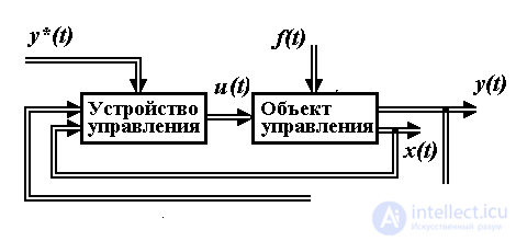
Fig. 4.7. The structure of the automatic control system

Local-level control systems provide a solution to the problems of stabilization, tracking, terminal control, etc. (see § 1.4.1), which provides for the maintenance of the specified laws of change of the controlled variables y ( t ) or state variables x _i ( t ). The control providing the decision of local tasks, is carried out by means of the regulator and the specifying block. The regulator calculates the ACS control signals based on the analysis of the current values ​​of the output variables y ( t ) and / or state variables x _i ( t ), as well as the corresponding driving effects y * ( t ) and / or x _i * ( t ) coming from environment or generated by the master unit (see. p. 4.2).

4.3.1. Principles of management. With the help of regulators, the contours of direct and feedback links are introduced into the control system. Depending on the structure of relations, there is a classification of management principles, shown in Fig. 4.8.

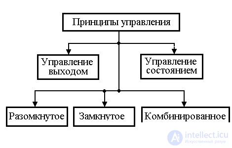
Fig. 4.8. Management principles

An attempt to directly solve local problems leads to control on the output of the OS and the simplest (classical) structure of the automatic control system containing the outlines of direct connections on the given influence u * and feedback on the output y . In this case, open, closed, and combined controls are distinguished. The latter two types provide for feedback on deviation.

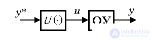
An open control introduces into the system a loop of direct communication for a given action:

(4.68) u = U ( y * ),

where U (·) is a functional operator. The control action is calculated from the condition of obtaining a given law of change in output (setting effect y * ( t )), and the current behavior of the OU is not controlled. The difference in the properties of a real object from its mathematical model used in constructing the algorithm (4.68), the possible instability of the control and the influence of perturbations usually lead to nonidentity of the output y ( t ) and the driving effect y * ( t ), i.e. errors of open-loop control systems (see § 2.3.2).

The deviation control introduces a feedback loop into the system structure:

(4.69) u = K ( ),

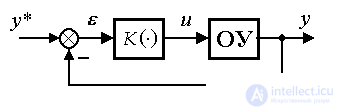
where is the mismatch (deviation) calculated by the formula:

(4.70) = y * - y ,

and the operator K (·) is chosen from the condition of reducing the deviation ( t ) during system operation. Since in this case, the behavior of the OS is adjusted depending on the current value , then the deviation control ensures the stability of the system and the reduction of the influence of disturbances (see § 2.3.2).

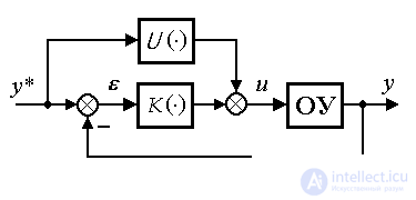
The absolute accuracy of the solution of the control problem can be achieved with the help of a combined control involving the use of both direct and reverse links:

(4.71) u = U ( y * ) + K ( ).

In some cases, the structure of the system is also supplemented by control loops for disturbing influences f , which provides compensation for the disturbing influence of the external environment.

The control systems of single-channel objects, built according to the classical principles of control over the output variable, contain no more than one feedback loop and therefore conditionally belong to single-loop systems .

Connecting additional feedback loops in multiloop systems provides improved control quality. The most complete information about the controlled process is contained in state variables (see clause 3.1.1), and therefore state-of-a-state management allows to achieve the best quality indicators of the management system.

In the state control, as well as in the output control, there are open-loop algorithms of the form

(4.72) u = U (x *),

representing the contours of direct links on the specifying effect x * ( t ), closed control algorithms (contours of feedback links on deviation):

(4.73) u = K (e ),

where the vector of mismatches (deviations) e is calculated by the formula:

(4.74) e = x * - x ,

and combined algorithms :

(4.75) u = U (x *) + K (e ).

The main functional element of the control device is the regulator. In accordance with the considered principles of control (see Fig. 4.8), there are output controllers and states, open controllers and combined-type controllers. Depending on the functional operators U () and K (), found in algorithms (4.68) - (4.71) or (4.72) - (4.75), there are:

• l inline and non-linear regulators;
• regulators with constant and variable parameters.

The further presentation concerns only linear regulators and, accordingly, linear closed control systems.

To describe the individual units of the system, differential and operator equations are used. Models of the system as a whole are found as the combination of blocks using well-known transformation rules (including the methods for transforming transfer functions, see § 2.4.1) and can be obtained in

• operator view corresponding to the input-output description;
• in the form of scalar or vector-matrix differential equations - input-state-output models.

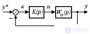
4.3.2. Output controllers and models of single-circuit systems. A single-loop system is the simplest and most common type of system that provides control of the output variable of a single-channel OU. The control unit of the single-circuit automatic control system includes the master unit BZ and the output regulator P (Fig. 4.9). The task of the system is to minimize the deviation = y * - y, which is prevented by the perturbation f ( t ) and nonzero initial mismatches ( 0 ) = ₀ The problem is solved with the help of output controllers .

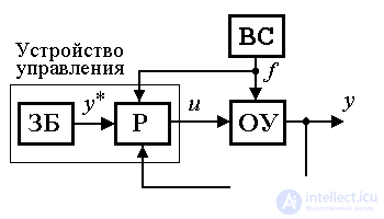
Fig.4.9. Single circuit system

Consider the properties of a linear object control system described by an operator equation

(4.76) ,

where W _О ( p ) is the OU transfer function, with various types of output regulators.

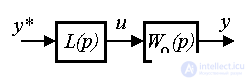
Open-type regulators are represented by a direct connection circuit for a given effect, i.e. by algorithm

(4.77) ,

where p = d / dt is the differentiation operator, - integro-differential operator (transfer function of the regulator). After substituting (4.76) into (4.77), we obtain an equation of the form

(4.78) ,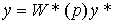

where W * ( p ) is the transfer function of the open-loop system

(4.79) .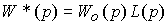

We introduce the tracking error (4.70) and substituting (4.70) into (4.78), we obtain the equation relating the specifying influence y * and the error " (error model):

(4.80) .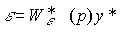

Integral-differential operator

(4.81)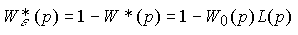

is called the transfer function (open-loop system) by tracking error . Choosing the transfer function of the regulator as

(4.82)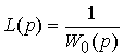

will get = 0 and therefore

(4.83) y ( t ) = y * ( t ).

Thus, the appropriate choice of the structure of the controller (4.77) allows to ensure the absolute accuracy of the solution of the tracking problem. The disadvantages of open-loop systems are indicated in § 4.3.1 and, in addition, are associated with difficulties in the practical implementation of the operator (4.82).

Closed regulators ( deviation regulators) introduce mismatch feedback into the system

(4.84) ,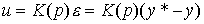

Where - integro-differential feedback operator (controller transfer function). Substituting (4.84) ​​into the OU equation (4.76), after the simplest transformations, we obtain the equation of the closed system

(4.85)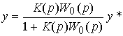

or

(4.86) ,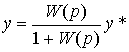

where W ( p ) is the transfer function of the open part of the system

(4.87) .

Equation (4.87) can be written as (see § 2.4.2)

(4.88) ,

Where - transfer function of a closed system

(4.89) .

Substituting (4.86) into equation (4.70) it is not difficult to obtain a tracking error model

(4.90)

or

(4.91) ,

Where - transfer function of a closed system by tracking error

(4.92) .

Note, (see also p. 2.4.2) that the closure of the system leads to a change in its transfer function (cf. expressions (4.76) and (4.92)) and, consequently, dynamic properties and accuracy indicators.

Depending on the private implementation of the operator there are proportional (P), proportional-differential (PD), proportional-integral (PI) and proportional-integral-differential (PID) controllers (see also 1.5.1):

P-regulators are described by an algebraic equation:

(4.93) ,

where K _p - constant feedback factor. The value of K _p is chosen in such a way as to reduce the magnitude of the deviation caused by the action of the perturbation f ( t ), the initial mismatch ₀ , and, possibly, by a high rate of change of the driving force y * ( t ). An increase in K _p usually provides a decrease in the error (see expressions (4.89) and (4.92) with K ( p ) = K _p )), but leads to a deterioration in the dynamic properties of the system — an increase in oscillation. Therefore, the problem of choosing the feedback coefficient is solved in a compromise manner.

To improve the dynamic properties of the ACS (reduce oscillation) in the control law introduce derivatives of deviations . Thus, the PD-controller algorithm is formed:

(4.94) ,

those. regulator with transfer function

(4.95) ,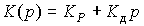

where K _d - the rate of feedback on the rate of change of error ( t ). The differential component of the algorithm (4.94) prevents the OU from moving rapidly and dampens vibrations. At the same time, a significant increase in the coefficient slows down the transient processes and, consequently, worsens the dynamics of the control system.

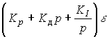
Improving the accuracy of the ACS (reducing the steady-state error   ) is achieved using a PI controller :

(4.96)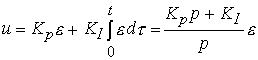

with transfer function

(4.97) ,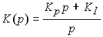

where K _I is the feedback factor for the integral of the error. The integral component of the algorithm (4.96) over time accumulates deviation information caused by the influence of the perturbation f and the rapid change in the reference y * ( t ), and thereby provides compensation for a possible steady-state error _y The increase in the coefficient K _I accelerates the processes of accumulation and compensation, but usually leads to system oscillations.

Simultaneous improvement of the dynamic properties and accuracy of the ACS is provided by the PID controller :

(4.98)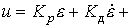

with transfer function

(4.99) ,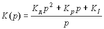

as well as more complex types of linear output controllers (4.84).

The use of deviation regulators is limited by a number of negative factors. First, the use of the differentiation operation is coupled with increased measurement noise and "noise" of the control channel. Secondly, the compensation of the disturbing influence of external influences f and y * requires certain time costs. Thirdly, for terminal control tasks (see § 1.4.1), in which the initial values ​​of the deviation are large, the control actions take unacceptably large values.

A more effective method of increasing the accuracy of ACS is proposed by linear regulators of the combined type , which contain, besides feedbacks on deviation, direct connections on the specifying effect:

(4,100) ,

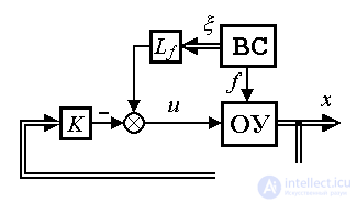
as well as communication on the disturbing effect (Fig. 4.10):

(4.101) ,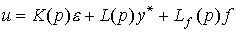

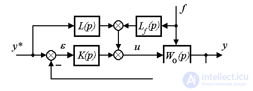
Fig. 4.10. Combined output control system

where L ( p ) and L _f ( p ) are the integrodifferential direct link operators.

Substituting the controller equation (4.100) into (4.76), we find the equation of a closed-loop system with a combined control

(4.102)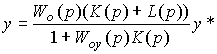

or equation (4.88), where the transfer function ( p ) takes the form

(4.103) .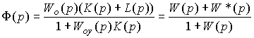

The tracking error equation is found as

(4.104)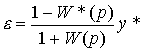

or in the form (4.91), where the transfer function closed loop by mistake tracking is like:

(4.105) .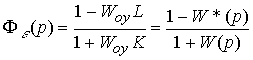

The choice of operators of direct links L ( p )   (and L _f ( p )) is carried out from the condition of compensation of the disturbing influence of the driving force y * (and, if necessary, the disturbance f ). With

(4.106)

as in the case of an open system, we get = 0 and therefore

y ( t ) = y * ( t ).

Таким образом, дополнение системы прямыми связями обеспечивает абсолютную точность ее работы ( = 0), а в функцию обратных связей (составляющей ) входит обеспечение заданных динамических свойств переходного процесса. При этом исчезает необходимость в подключении интегральных составляющих управления и оператор выбирается как оператор П- или ПД-регулятора.

Итак, модели одноконтурных систем легко получаются в операторном виде методами преобразования передаточных функций. Для невозмущенных моделей ( f ( t ) = 0) - это выражения (4.102) или (4.104). Аналогичные модели могут быть получены для систем с возмущением (см. п. 2.1.4).

4.3.3. Регуляторы и модели систем управления состоянием. Системы с регуляторами состояния относятся к многоконтурным системам и, следовательно, обладают лучшими точностными и динамическими свойствами, чем одноконтурные. Они используются для управления как одноканальными, так и многоканальными ОУ. Проанализируем системы с линейными регуляторами состояния в одноканальных задачах стабилизации и слежения (см. п. 1.4.1). В общем случае в состав модели ВСВ входит следующие блоки:

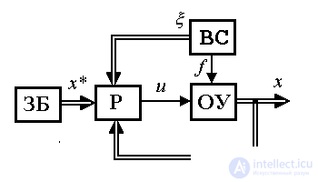
Fig. 4.11. Condition management system

• модель ОУ:

(4.107) ,

(4.108) ;

• задающий блок ЗБ (генератор задающего воздействия)

(4.109) ,

(4.110) ;

• модель внешней среды ВС (генератор возмущающего воздействия)

(4.111) ,

(4.112) ;

• регулятор Р, представленный одной из общих моделей вида (4.72), (4.73), (4.75).

Рассмотрим системы с наиболее распространненными типами регуляторов состояния.

Сначала проанализируем задачу стабилизации ОУ в точке x=x*= 0. Простейший регулятор состояния - пропорциональный (П-регулятор состояния, или модальный) регулятор - вводит обратные связи по переменным x _i . Алгоритм его работы описывается алгебраическим уравнением

(4.113) ,

где K - матрица-строка коэффициентов обратной связи

K= .

Алгоритм (4.113) можно записать в развернутой форме

(4.114) .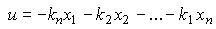

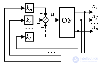
Выбор коэффициентов k _i матрицы обратных связей K обеспечивает получение заданных динамических свойств системы: быстродействия и колебательности.

Замечание 4.2. Для одноканального ОУ в качестве координат х _i вектора х можно выбрать фазовые переменные (см. 3.3). Тогда первые члены формулы (4.114) будут соответствовать описанию ПД-регулятора выхода (4.95) при задании y* = 0.

(4.115) .

Поэтому регуляторы состояния являются обобщением ПД - регуляторов, хотя и не содержат в явном виде дифференцирующих звеньев.

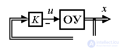
Рассмотрим простейший случай задачи стабилизации ОУ

(4.116) ,

в нулевой точке: . Воспользуемся пропорциональным регулятором (4.113). Замкнутая система принимает вид

(4.117) ,

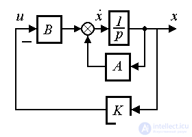
Fig. 4.12.A system with a proportional state controller where
= A-BK is a matrix of a closed system that determines the dynamic properties of a system with a proportional state controller.

Note that in the case under consideration (in the absence of disturbances) the controller (4.113) ensures the absolute accuracy of the stabilization of the system at a given point x * = 0.

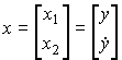
Example 4.4. For a second order object

(4.118)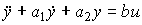

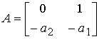
(see example 3.1) the model (4.116) takes the form

(4.119) ,

(4.120) 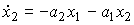+ bu ,

(4.121) ,

those.

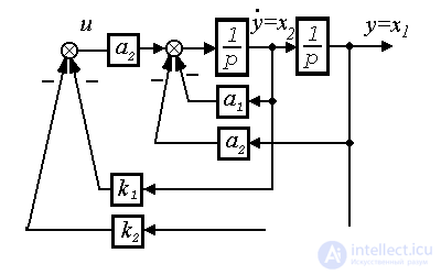
Fig.4.13. Second order system

, , .

Here the proportional control algorithm is

(4.122) ,

those.

.

The model of a closed system takes the form

(4.123)

or (4.117), where the matrix of the closed system is as

.

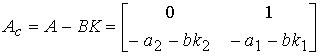Under the conditions of external disturbances at the OS, accuracy indicators of a system with a proportional state regulator are limited. The increase in steady-state accuracy is achieved by introducing integral feedback links into the control loop. The PI state controller implements the algorithm:

(4.124) ,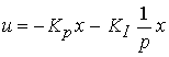

where K _I is the matrix of feedback coefficients for the integral of the state vector. The integral component of the algorithm (4.124) over time provides partial or full compensation of the disturbance f ( t ).

Комбинированный регулятор состояния позволяет обеспечить компенсацию возмущения за счет прямых связей по возмущению f ( t ). Отметим, что наилучшие результаты могут быть получены при использовании достаточно полной информации о возмущении, что соответствует введению прямых связей по вектору состояния внешней среды ( t ):

(4.125) ,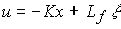

где L _f - матрица прямых связей. Во многих случаях вектор , составлен из возмущения f и его производных.

Задача слежения рассматривается как задача отработки расширенного вектора задания x* ( t ). П-регулятор состояния в подобных следящих системах вырабатывает управляющие сигналы, пропорциональные вектору отклонения е = х*-х , т.е. описывается уравнением

(4.126) .

Алгоритм (4.126) можно записать в развернутой форме

(1.27) u= ,

Where

(4.128) .

Замечание 4.3. В качестве координат х _i вектора х можно выбрать фазовые переменные (см. замечание 4.2), а в качестве координат вектора x* - функции . Then

(4.129)

и первые члены формулы (4.127) будут соответствовать описанию ПД-регулятора выхода (4.94):

(4.130) .

ПИ-регулятор состояния дополняет структуру системы интегральными связями и описывается выражением

(4.131) .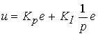

Интегральная составляющая алгоритма (4.131) обеспечивает c течением времени частичную или полную компенсацию возмущающего влияния задающих воздействий и возмущений.

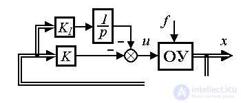
Эффективная компенсация отклонений, вызванных возмущением f ( t ) и текущими вариациями задания x* ( t ), достигается при использовании комбинированного алгоритма управления (рис. 4.14)

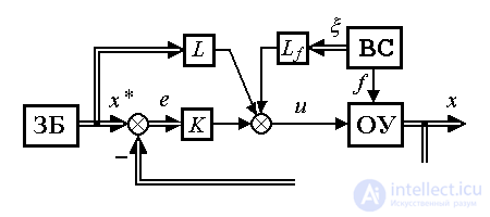
Fig. 4.14. Комбинированная система управления состоянием

(4.132) .

Замечание 4.4. В отличие от регуляторов выхода большинство алгоритмов управления состоянием (алгоритмы (4.113), (4.125), (4.126), (4.132)) не используют динамических операторов, что обеспечивает их более простую практическую реализацию.

Рассмотрим задачу стабилизации невозмущенного ОУ (4.116) в произвольной точке: . Задача сводится к задаче слежения, где задающий блок представлен уравнением

(4.133)

с начальным значением x* (0) = x* . Воспользуемся пропорциональным регулятором (4.126). Модель ошибки получается дифференцированием по времени выражения (4.74) и подстановкой уравнений (4.116) и (4.109):

(4.134) .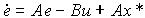

Она имеет структуру возмущенной модели (4.107), где роль возмущения играет компонента Ax* . При использовании пропорционального регулятора

(4.135) ,

модель ошибки (4.134) принимает вид

(4.136) ,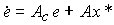

Where - матрица замкнутой системы. Если det A _c 0, из условия получим значение уставившейся ошибки (см. п. 3.2.3)

(4.137)

и, следовательно, пропорциональный регулятор не обеспечивает абсолютной точности решения рассматриваемой задачи.

При использовании комбинированного регулятора

(4.138) ,

модель ошибки (4.134) принимает вид

(4.139) .

Если матрицу прямых связей L выбрать так, чтобы

(4.140) ,

Fig. 4.115. Комбинированная система стабилизации состояния

то уравнение ошибки принимает вид

(4.141) .

Из последнего уравнения видно, что e _у = 0 и, следовательно введение прямых связей по задающему воздействию обеспечивает в установившемся режиме абсолютную точность стабилизации

x=x*.

Итак, модели систем управления состоянием получаются как совокупность динамических моделей объекта управления, задающего блока, внешней среды и регулятора. Простейшие преобразования позволяют получить уравнения замкнутых моделей состояния, а при необходимости, моделей ошибок стабилизации (слежения).