Lecture
The system of automatic control in the course of work can be in one of two, qualitatively different from each other, states: in steady or unsteady modes.
The steady-state (normal) mode of operation of an automatic system is characterized by the invariance of the external conditions of the system.
Unsteady (transient) mode of operation occurs immediately after exposure to a system of control or disturbing signals. The behavior of the controlled variable in the unsteady mode is called transient . Transients can be fading and non-fading. With a fading transient, the controlled variable tends to its state in the steady state.
In a system with a non-damping transient, the regulated quantity either increases indefinitely (most often in the form of diverging oscillations) or remains in the same state as at the beginning of the transient process. Such a system never comes into a steady state set for it and is called unstable.
Typical input signals used in the study of automatic systems
To study the transients of an automatic system, it is necessary to apply such an impact to the system input that would take it out of the state of rest and subsequently provide free movement of the controlled quantity. Such input influences are step function and impulse? - function (Dirac function) (Fig. 4.1, Fig. 4.2).
A single step function is denoted by 1 (t) and is an expression:
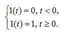 (4.1)
(4.1)
Function 1 (t) is continuous everywhere, except for the point t = 0, where it suffers a discontinuity of the first kind. This function corresponds to the closure of a switch that supplies a voltage of 1 volt. The image of the single function according to Laplace is:
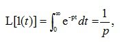 (4.2)
(4.2)
To record an arbitrary step signal, use the expression
x (t) = Al (t) (4.3)
where A is the signal amplitude.

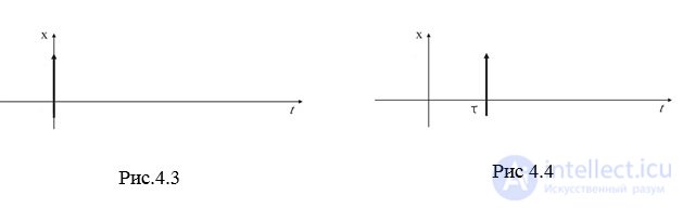
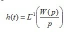
Pulsed? - a function is a function that is equal to zero everywhere, except the origin, where it is equal to infinity (Fig. 4.3, Fig. 4.4):
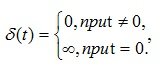 (4.4)
(4.4)
The integral of this function over any interval containing the origin is equal to one, i.e.
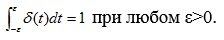 (4.5)
(4.5)
The impulse function is a mathematical idealization of an extremely short pulse, whose area is equal to one. The image of the Laplace impulse function is:
 (4.6)
(4.6)
Impulse? - the function is derived from a single step function
 (4.7)
(4.7)
Pulse? - the function has a filtering property.
The reactions of an automatic system to a single step function and a pulse function are called the temporal characteristics of the system, since they represent the process of changing the controlled variable over time.
Time characteristics
The type of the transition process, the quality of regulation and the state of the automatic system in a steady state are determined by the type of transition and weighting functions (characteristics) of the system.
The transition characteristic of a linear automatic system is its response to the action of a single step function with zero initial conditions.
The transient response is denoted by h ( t ) and is a transient process caused by an abrupt change in the input quantity. It can be determined by solving a differential equation by an ordinary or operator method.
 (4.8)
(4.8)
The weight function of a linear automatic system is called its response to a pulse? - function with zero initial conditions.
The weight function is denoted by k ( t ) and is a transient process caused by the instantaneous “shock” effect of a short pulse at the system input. The weight function is also found by solving the differential equation of the system.
 - weight function (4.9)
In the study of the dynamic properties of an automatic system of interest are:
- system behavior at the initial moment of time (immediately after the application of the impact);
- the nature of the change of the regulated value in a transient mode;
- behavior of the regulated value when approaching a new steady state;
- the behavior of the controlled variable in steady state;
- the duration of the transition process.
Information about this can be obtained by analyzing the weight or transition functions of an automatic system.
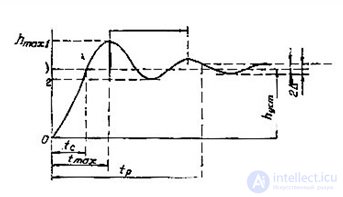
Fig. 4.5. Transition curve
1) The regulation time t p is the minimum time after which the controlled variable will remain in a fairly small neighborhood of the steady-state value, i.e.
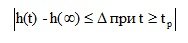 (4.10)
where - a constant value, the value of which is usually taken 5%.
2) The absolute and relative magnitude of the overshoot, determining the deviation of the transient response from the steady-state value.
 (4.11)
and the relative deviation, expressed as a percentage,
 (4.12)
3) The time of the first negotiation (speed) t c , which determines the time of the first achievement of the steady-state value of h (?).
4) Oscillation frequency  - the period of oscillation of the transient response.
5) The number of oscillations n, which has a transient response during the regulation time t p .
6) The time to reach the first maximum t max .
In any automated control system, as a result of the action of disturbing forces, on the one hand, and the restoring action of the control device, on the other hand, a transient occurs: the transition of the automatic control system from one state to another. Consider the different types of transition process (Fig. 4.6).
The solution of a differential equation describes the transition process y (t), the nature of which is determined by the coefficient. Consider transients corresponding to different values.
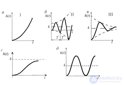
Fig. 4.6
four. ? > 1. The characteristic of the system is the same as in the third case, but the transient process is monotonic (aperiodic) (Fig. 4.6, d).
5.? = 0; A periodic motion is established in the system, the process is called oscillating continuous, the system is on the stability boundary (Fig. 4.6, e). It is closed (conservative), autonomous from the external environment.
All considered oscillations (II, III and V cases) belong to the class of free ones, their parameters are A and? depend on the initial conditions, i.e. from the introduced energy. For cases II and III, the function is h (t) h h (t + T), where T is the oscillation period, and therefore, these oscillations are non-periodic. Periodic oscillations are observed only in the case of V
Example 1. Given the equation in differential form:
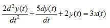
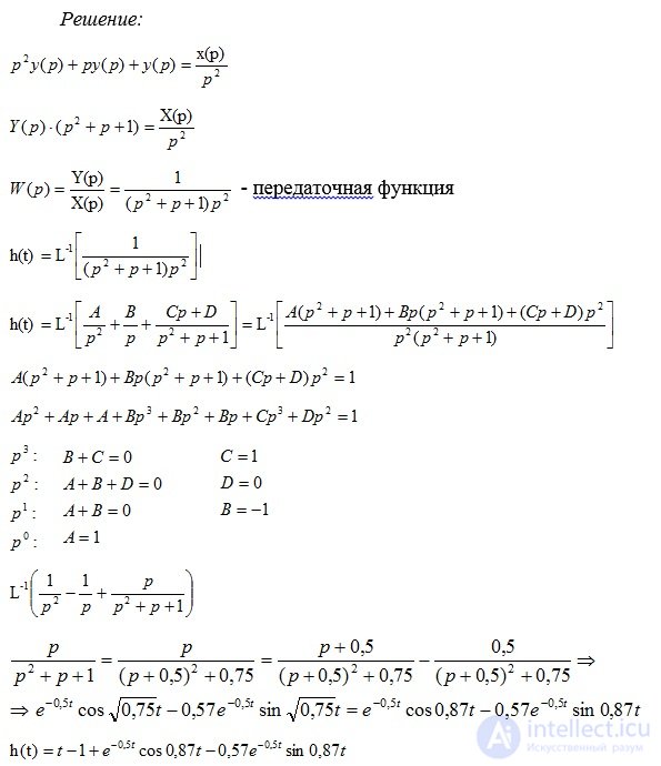
Determine the transient and weight characteristics. Build graphics.
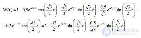
Decision:
The transient response is determined by the formula (4.8):
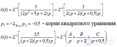
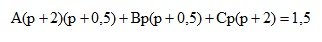
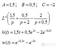
A, B, C are determined using the method of uncertain coefficients.

Equate the numerators of two fractions
Laplace weight function
Attention!
The solution uses the method of uncertain coefficients (from the course of higher mathematics). The method of undetermined coefficients is used when integrating rational fractions. A rational fraction is a fraction of the form.
 ,
,
where P ( x ) and Q ( x ) are polynomials. A rational fraction is called correct if the degree of the numerator P ( x ) is lower than the degree of the denominator Q ( x ) ; otherwise, the fraction is called improper. Any correct rational
A fraction can be uniquely represented as a sum of simple rational fractions. Simple rational fractions:
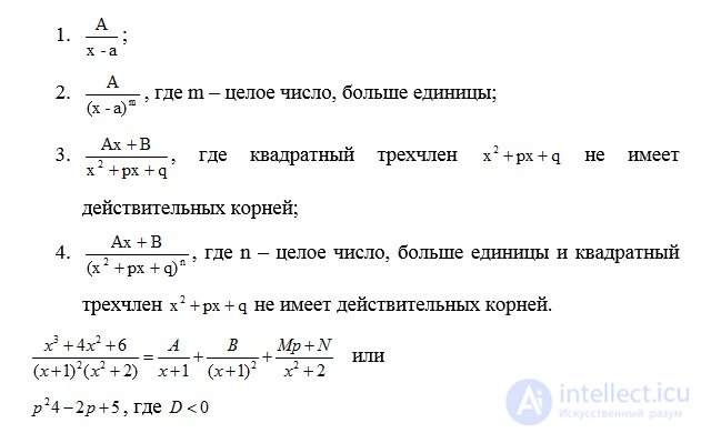
If when solving differential equations:
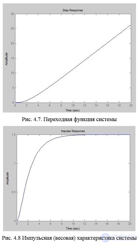
Conclusion: According to the obtained transition function, we can conclude that the system is unstable.
Example 2. An operator is defined for a linear stationary system 

Conclusion: According to the obtained transition function, we can conclude that the system is unstable.

Comments
To leave a comment
Mathematical foundations of the theory of automatic control
Terms: Mathematical foundations of the theory of automatic control