Lecture
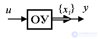
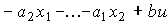
3 .2.1. Models input-state-output. First, we consider a particular case of a controlled dynamic system with one input u ( t ) and one output y ( t ), described by the equation [M1a], where a 0 = 1. We introduce state variables (3.1). Differentiating (3.3) in time and substituting [M1a], we find the equation of state:
(3.38) 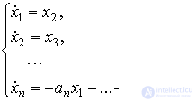
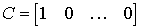
In this case, the output equation still has the form (3.8). Equations (3.38) and (3.8) are the simplest case of the input-state-output (VSB) model.
In the more general case, the model BC of the controlled dynamic system [M1] contains the equations of state of the form:
[M4] 
and the output equation [M5]. To convert them to a compact vector-matrix form, it is necessary to determine the state vector  ,
,  matrices
  ,
,  as well as size entry matrix

 .
.
Then the equations [M4], [M5], describing the model input-state-output, take the form:
[M6]  ,
,
[M7]  ,
,
Where  .
.
Model [M6] and [M7] connects the input  and exit
  through intermediate variables
  .
.
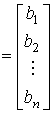
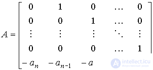
In the particular case, when the model ENE is presented in the form (3.38), (3.8), we obtain the matrix
 ,
,  ,
,  .
.
Similarly, we obtain a model of a VSV multichannel (multiply connected) system (see model [M2m]). In general, it contains the equations of state of the form
[M4m] 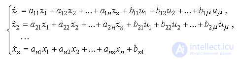
and output equations [М5m]. Define  -dimensional control vector:
 and m- dimensional vector of outputs
 as well as matrices
 ,
, 
dimensions  and
and  , respectively. Then the equations [M4m] and [M5m] can be rewritten as [M6] and [M7].
Consider a perturbed dynamic system, (see [M1f]), i.e. controlled system to the input of which the input signal additionally acts (disturbance)  ( t ). The equation of state of such a system is written in the form:
[M4f] 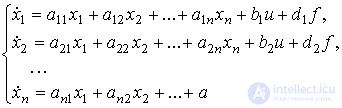 ,
,
where d i ,  , are the coefficients, and the output equation preserves the form [M5]. The vector matrix form of the model [M4f] is:
[M6f] 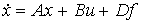 ,
,
[M7] y = Cx ,
Where 
 .
.
If several disturbing influences f k act on the input of the system, then in the equation [M6f]  - vector of perturbations, and
  .
.
In the particular case (see (3.35)), the equations of state of the perturbed system take the form
(3.39) 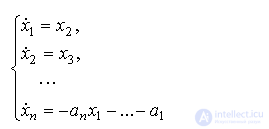
and in the equation [М6f]
 .
.
Consider solutions of equations [M6], [M7], assuming  . The solution of the equation of state [M6] can be represented as:
(3.40)  ,
,
Where  ( t ) is the free component ( transition process of an autonomous system), corresponding to the solutions of the homogeneous differential equation [M6a] and depending on the initial conditions
  ,
,  ( t ) - forced component corresponding to the transition process of the system [M6] with zero initial conditions
  (system response to the input action u ( t )).
Substituting (3.40) into the output equation [M7], we get
(3.41) 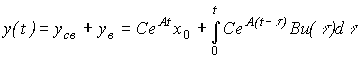 ,
,
Where
(3.42) 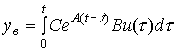 .
.
Note that the matrix
(3.43) 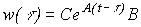
is a weight (pulse transient) matrix (with  - the weight function) and, therefore, the equation (3.42) coincides with the previously given expression (2.35).
For perturbed models, the NER solutions can be obtained in a similar form.
3.2.2. The transfer function (matrix) of the model BCB and block diagrams. The above equations describing the input-state-output models can be written in operator form (see 2.1). Consider the equations [M6a], [M7]. Using the differentiation operator p = d / dt , we write  . Then from the equation of state [M6a] after the simplest algebraic transformations we find
(3.44)  .
.
Substituting the last expression into the output equation [M7] we get
(3.45) 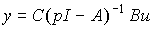 .
.
We introduce the notation
(3.46) 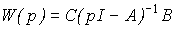
and write the previous equation in the form
(3.47)  .
.
Comparison with the equation [M3m] shows that the matrix integro-differential operator W ( p ) is nothing but the transfer matrix of the controlled dynamic system (see § 2.1.3).
Consider the properties of the operator (3.4 6). Matrix  is called resolvent and can be represented as
(3.48) 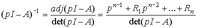 ,
,
Where  - numeric matrices
  . Then
(3.49) 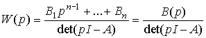 ,
,
Where  ;
;  - matrix operator.
For the case of a single-channel system ( m = = 1) W ( p ) - transfer function. Taking into account equation (3.48), we find that
(3.50)  -
-
characteristic polynomial of the system; but
(3.51)  -
-
characteristic polynomial of the right side of the differential equation (see § 2.1.1). Consequently, the eigenvalues of the matrix A coincide exactly with the roots of the characteristic equation (poles) of the system
(3.52)  .
.
To build a structural scheme corresponding to the model of BCB, we rewrite the equation of state [М6] in the operator form
(3.53) 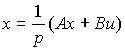
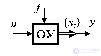
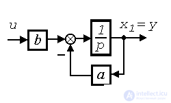
and also use the equation of output [M7]  . The block diagram of the system takes the form shown in Fig. 3.2.
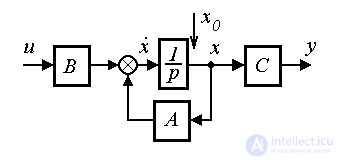
Fig. 3. 2. The block diagram of the model ENE
In the particular case when the equations of state are written in the form (3.38), (3.8) we find
(3.54) 
(3.55) 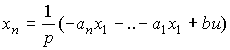 .
.
Fig. 3.3. Block diagram of the model (3.38), (3.8)
The structural diagram is shown in Fig. 3.3 and corresponds to the cononically controlled form of the linear system representation (see § 3.3.2)
3.2.3. Static mode Consider the behavior of the model ENE with a constant input (control) effects, i.e.  . In this case, the solution of the differential equation [М6а] corresponds to the established component of the transition process and is sought in the form
 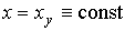 . Noticing that
  we find:
(3.56) 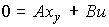 .
.
Provided that  (i.e.
(i.e.  ), the algebraic equation (3.56) is uniquely solvable for x y :
(3.57) 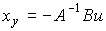 .
.
Substituting the found solution into the output equation [M7], we find the static characteristic of the system [M6a], [M7]
(3.58) 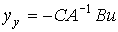 .
.
Taking into account the expression (2.47), we can clearly write
(3.59) 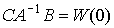
and get the expression (2.46).
If the system is such that  , then matrix A is irreversible and the system does not have a static mode (see § 2.2.5).
Example 3.1. Consider a second-order system ( n = 2), the explosive model of which is represented by the equation
(3.60) 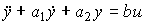 .
.
State variables are defined by expressions.
(3.61)  ;
; 
and model BCB are both
(3.62) 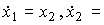
 ,
,
(3.63)  .
.
The vector matrix form of the model is
(3.62a) 
 ,
,
(3.63a)  .
.
Example 3.2.  - the circuit considered in clause 1.1.2 is described by a differential equation of the first order:
(3.64) 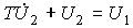 .
.
We introduce the notation
(3.65) 
and
(3.66)  .
.
Equation (3.64) takes the form
(3.67) 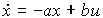 ,
,
(3.68)  ,
,
Where  and
and  .
.
Example 3.3. Consider a second order differential equation
 ,
,
describing the motion of a material point (see example 2.3).
The equation is reduced to
(3.69)  ,
,
Where  . We introduce state variables
(3.70)  ,
,
(3.71) 
and find a model of VSV as
(3.72)  ,
,
(3.73) .
The vector matrix form of the model is
 ,
,
.
This is a special case of the previously considered model (3.62a), (3.63a).

Comments
To leave a comment
Mathematical foundations of the theory of automatic control
Terms: Mathematical foundations of the theory of automatic control