2.4 Building Input / Output Models

The input-output model of the control system is based on the known equations of individual components (blocks, links, see Section 4.1). The procedure reduces to transforming a system of differential equations describing the behavior of individual blocks to a single equation of a control system of the form [M1], [M2] or [M3]. At the same time, regardless of the initial description, the operator form [M3], which at the end of the procedure can be easily reduced to the form [M1] or [M2], is most convenient for implementing such transformations.

2.4.1. The simplest connection blocks. Consider the sequential connection of blocks, i.e. the system consisting of blocks B1 and B2 and described by operator equations:

(2.82) ,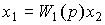

(2.83) ,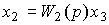

where respectively - day off, and - system input signals.

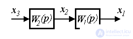
Fig. 2.18. Serial block connection

It is required to find a unified description of the system (2.82) - (2.83), i.e. the equation of connection of signals and . Substituting (2.83) into (2.82) we get

(2.84) .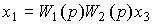

Thus, the system is described by the equation

(2.85) ,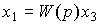

Where 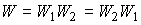- the transfer function of the system of series-connected blocks.

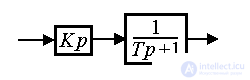
Example 2.4. Consider the serial connection of aperiodic link (with a single transmission coefficient) and an ideal differentiating link (see p.2.3). The application of the rule discussed above gives the transfer function

(2.86) ,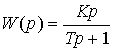

which coincides with the transfer function of a real differentiator.

Consider a parallel connection of the same blocks, i.e. system described by equations

(2.87) ,

(2.88) ,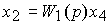

(2.89) ,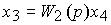

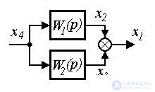
Fig. 2.19. Parallel block connection

Where - day off, and - system input signals. After appropriate substitutions find the connection output and input:

(2.90) ,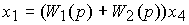

or

(2.91)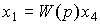

Where 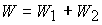- transfer function of a system of parallel-connected blocks.

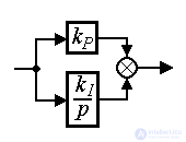
Example 2.5. Consider a parallel connection of proportional and integrating links (PI controller, see p. 4). Using the rule obtained above, we find the transfer function of a link, called isodrome:

(2.92) .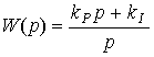

Consider a system composed of two blocks, one of which is connected to the other in the form of negative feedback ( connection to feedback ), i.e.

(2.93) ,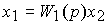

(2.94) ,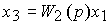

(2.95) ,

Where - day off, and input - system signal.

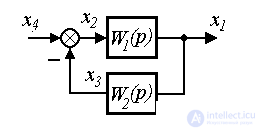
Fig. 2.20. Connection to feedback

After elementary transformations, we get

(2.96) .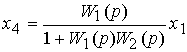

Thus, the system is described by an equation of the form (2.96) and has a transfer function

(2.97) .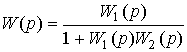

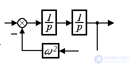
Example 2.6. Consider a double integrator having a transfer function

,

with negative feedback, formed by a proportional link with a coefficient 2 Using the formula (2.96) we find

,

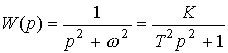where k = 1 / 2 , T = 1 / i.e. the composite unit is a conservative unit (see § 2.5).

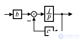
Example 2.7. Consider a serial connection proportional link with the coefficient b and the integrator with negative feedback in the form of a proportional block with a factor a . Using the rules discussed above we find

(2.98) ,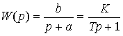

where a = K / T, b = 1 / K. The resulting transfer function corresponds to an aperiodic link (see § 2.3).

Note that for a system with positive feedback, equation (2.95) takes the form

(2.99)

and

(2.100) .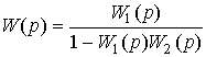

On the other hand, in the simplest particular case (a single negative feedback ) and therefore

(2.101) .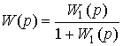

2.4.2. Transfer functions of control systems. First, we consider an open-loop control system (the so-called open-loop system, see Section 4.3), consisting of a series-connected controller and control object. Let the control object be described by the operator equation

(2.102) ,

and the controller is represented by the expression

(2.103) ,

Fig. 2.21. Open system

where y ( t ) is the output variable, u ( t ) is the controlling action, y * ( t ) is the specifying action (system input), W 0 ( p ) and K ( p ) are the transfer functions (intergro-differential operators). Using the rule for constructing a model of series-connected blocks, we find the equation

(2.104) ,

connecting the output variable y ( t ) and the input variable y * ( t ) through the transfer function of an open-loop system

(2.105) .

The transfer function can be written as

(2.106) ,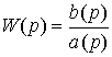

where a (p), b (p) are differential operators of corresponding degrees. Then equation (2.104) can be reduced to

(2.107)

and, if necessary, rewrite in standard form [М1].

Now consider the closed control system, i.e. the system represented by the control object (2.102) and the simplest deviation regulator (see section 1.5):

(2.108) u ( t ) = K ( p ) e ( t ) ,

(2.109) e ( t ) = y * ( t ) - y ( t ) ,

where e is the mismatch (error). Using rule (2.96) we find the model of a closed system in the form

(2.110) ,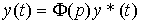

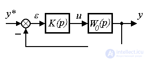
Fig. 2.22. Closed loop system

Where ( p ) - the transfer function of a closed system, defined as

(2.111) .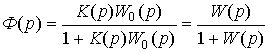

Given (2.106) it is not difficult to get

(2.112) .

Comparing the last expression with (2.106) shows that the closure of the system leads to a change in the denominator of its transfer function a ( p ) + b ( p ), i.e. characteristic polynomial system.