Fourier and Laplace transforms.

Fourier transform

Ratio

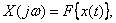
called the direct Fourier transform. Corner frequency function - called the Fourier transform or frequency spectrum function . The spectrum characterizes the ratio of the amplitudes and phases of an infinite set of infinitely small sinusoidal components, which together form a non-periodic signal . The Fourier transform operation is mathematically written as follows:

Where - the symbol of the direct Fourier transform.

The spectra in the theory of automatic control are represented graphically, depicting separately their real and imaginary parts:

In fig. 1 shows a typical image of the spectrum of a non-periodic signal.

Fig. one

We note the following features of the spectrum of a non-periodic function :

1. The spectrum of the non-periodic function of time is continuous;

2. The range of valid values ​​of the spectrum argument

1. The real part of the spectrum is an even frequency function, the imaginary part of the spectrum is an odd function, which allows using one half of the spectrum

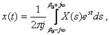
The Fourier transform is reversible, that is, knowing the Fourier image, you can determine the original function - the original. The ratio of the inverse Fourier transform is as follows:

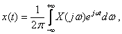
or in abbreviated notation where - the symbol of the inverse Fourier transform. Note that a time function has a Fourier transform if and only if:

• the function is unambiguous, contains a finite number of maxima, minima and discontinuities;

• the function is absolutely integrable, i.e.

The inverse Fourier transform is only possible if all poles - left.

Consider the examples of determining the spectrum of temporal functions.

Example :

Find the frequency spectrum of the delta function.

,

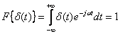as when

,

and at and

.

Eventually, has a single, uniform and frequency independent real spectrum, and the imaginary part of the spectrum will be zero (see Fig. 2).

Fig. 2

Example :

Let us find the frequency spectrum of a single step function.

For this function, the requirement of absolute integrability is not fulfilled, since

therefore Fourier image has not.

Laplace transform

Ratio

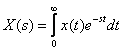
called the direct Laplace transform. Complex variable called the Laplace operator, where - angular frequency, - some positive constant number. Complex variable function called signal image according to Laplace. The operation of determining the image from the original is abbreviated - where - the symbol of the direct Laplace transform.

The Laplace transform is reversible, that is, knowing the image from Laplace, you can determine the original using the ratio of the inverse transform

or 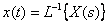where - the symbol of the inverse Laplace transform.

Note that the Laplace transform represents the original function only when , and the behavior of the original function when no effect on the image. The class of functions transformed by Laplace is much wider than the class of functions transformed by Fourier. Virtually any time functions in TAU have a Laplace transform.

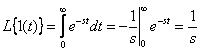
We obtain Laplace images for impulse functions.

,

because at ,

and at .

.

In practice, the conversion tables are used to perform the direct and inverse Laplace transformations, a fragment of which is shown in Table. one.

Table 1.

The Laplace transform tables can be used to determine the Fourier transforms of such absolutely integrable functions that are 0 for . To obtain Fourier images in this case, it suffices to put Laplace in the image . In general, it looks like

,

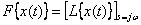if a at and

Consider the statements of the main theorems of the Laplace transform, which are widely used in TAU.

1. The linearity theorem. Any linear relation between the functions of time is also valid for the Laplace images of these functions;

;

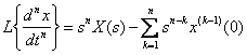
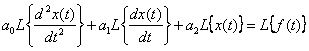
1. The differentiation theorem of the original.

If a and then ,

Where - the initial value of the original.

For the second derivative, use the expression

.

For derivative th order is true the following relationship:

;

For derivative th order with zero initial conditions, the following relationship holds:

;

i.e. differentiation degree of the original in time with zero initial conditions corresponds to multiplying the image by .

1. The original integration theorem.

;

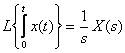Comment

In the field of images according to Laplace, the complex operations of differentiation and integration are reduced to the operations of multiplication and division by that allows you to move from differential and integral equations to algebraic. This is the main advantage of the Laplace transformation as a mathematical tool of the theory of automatic control.

1. Delay theorem. For anyone fair value

;

1. The convolution theorem (multiplication of images).

,

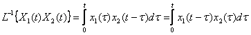Where

;

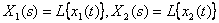1. Limit value theorem. If a then

if a exists.

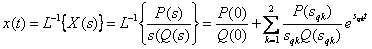
To find the original function in its image using the inverse Laplace transform. The image function must be represented in the form of Heavisite, using the necessary formula for the decomposition of a fractionally rational function. The resulting sum of the simplest fractions is subjected to the inverse Laplace transform. To do this, you can use the Laplace transform tables, which define the images of many temporary functions. A fragment of the Laplace transform table is given in Table. 1. In cases where there are complex conjugate poles of the image, it is necessary to convert the corresponding simple fractions into a form suitable for using the Laplace transform table. The use of a personal computer with packages of mathematical programs containing the functions of the direct and inverse Laplace transformations makes it much easier.

Example

Define the original in the image as a fractional rational function

.

We use the Hevisite decomposition for a fractional rational function with one zero pole. Then

.

Decomposition coefficients are

.

The image in the form of Heavisite has the form

.

We use the linearity theorem and the transformation table for each term, as a result we get

.

The graph of the original function has the form shown in Fig. 3

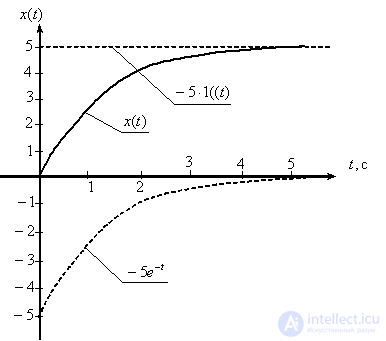
Fig. 3

We briefly explain the algorithm for solving differential equations by an operator method using the example of solving a differential equation of order 2 in general

,

Where , , .

We apply the differentiation theorem to find images of derivatives

, .

Let be then

.

We obtain an operator equation using the linearity theorem

,

.

Solve the equation for ,

.

We find using the transition to the Heavisite form (decomposition of Heavisite)

,

Where , .

Particular attention should be paid to obtaining the image of the derivative of the step unit function. which is defined as follows:

If use

,

This is an erroneous solution, so you should use the “left” initial conditions called

.

The validity of this can be easily verified by substituting the solution into the original differential equation.

Test questions and tasks

1. What restrictions are imposed on the direct and inverse Fourier transforms?

2. How to get the frequency spectrum of a real signal - a non-periodic function of time using the Laplace transform tables?

3. If the image according to Laplace has the form of a fractionally rational function, in what form is it more convenient to represent it for obtaining the original, in the form of a Bode or in the form of Hevisite?

4. Determine the original image of the following Laplace

.

Answer :

.

1. Determine the original image of the following Laplace

.

Answer :

.

1. Find solving a differential equation

,

Where .

Answer :

.

1. Find solving a differential equation

,

Where .

Answer :

.