Lecture
Any control system is a combination of several devices in which phenomena of different physical nature occur. The same system may include, for example, mechanical, electrical, pneumatic and hydraulic elements.
Consider the elements in which energy conversion processes are strictly oriented, that is, energy and effects are transmitted only in a certain direction, have a detecting property. This means that the output value of the element does not affect its input.
Usually, the elements of a system that transmit informational influences have the property of one-pointedness. These elements include gauges and signal converters.
The first step in the study or design of a control system is the compilation of a mathematical description of its elements and the system as a whole.
The compilation of a mathematical description of a structural element of a control system consists of the following successively performed procedures: the adoption of certain assumptions, the choice of input and output variables, the choice of a reference system for each variable, the application of a physical principle that reflects in mathematical form the laws of energy or substance conversion.
An automatic system of 1 input and 1 output is called linear if its operator satisfies the superposition principle, which is expressed by the following equation:
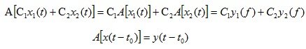 (1.1)
(1.1)
An automatic control system (hereinafter referred to as an ACS) is called stationary, if the shift of an arbitrary input signal x (t) at any time t 0 is accompanied by the same shift of the output signal y (t), then it is true:
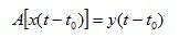 (1.2)
(1.2)
The operator of a one-dimensional ACS is a rule that defines a single output signal for any given set of input signals y (t) = [x 1 , x 2 , x 3 , ...].
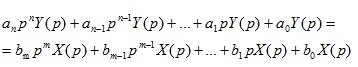
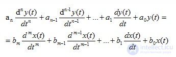
For an element that has one input X (t) and one output Y (t) signal, the ordinary differential equation is written in the general case as follows:
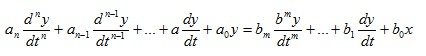 (1.3)
(1.3)
a, b - indirect coefficients of the system;
x, y - output and input signals;
n is the order of the output signal;
m is the order of the input signal.
This expression is also called the operator of a linear stationary system.
The equation is called the equation of dynamics or the equation of motion of an element. The concept of "movement" is used in the most generalized sense.
The equation can be linear and non-linear. In addition to the main variables, it includes constant values called parameters.
If in equation (1.3) the functions of time x (t), y (t) are replaced by functions of the complex variable X (p), Y (p), then it turns out that the differential equation will be equivalent to a linear algebraic equation:
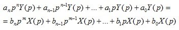 (1.4)
(1.4)
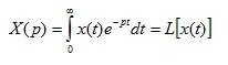
The Laplace transform is based on the following two formulas:
- direct Laplace transform
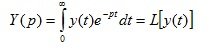 (1.5)
(1.5)
- inverse Laplace transform
 (1.6)
(1.6)
p is a complex variable, t is a time parameter
The transition from the original function y (t) to its image Y (p) is called the direct Laplace transform. The inverse Laplace transform is a transition operation from the image of the function to its original.
The transfer function W ( p ) is the ratio of the image in the Laplace output value to the image in the Laplace input value with zero initial conditions.
 (1.7)
(1.7)
Considering the linear differential equation (1.5) and finding the image for the left and right sides of the equation, we get
 (1.8)
(1.8)
From here
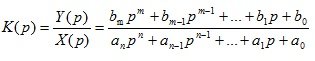 (1.9)
(1.9)
The transfer function, like the differential equation, fully determines the dynamic properties of the automatic system. Knowing the transfer function of the automatic system and the image of the input signal, it is easy to find the image of the output signal:
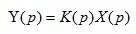 (1.10)
From expression (1.10), using the inverse Laplace transform, we get
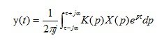 (1.11)
The transfer function does not depend on the type of input signal and is completely determined by the structure and parameters of the linear system.
Consider the basic properties of the transfer function. From the expression (1.9) it can be seen that in the general case the transfer function is a fractional rational function of the complex variable “p”. Denote
- polynom in the transfer function numerator:
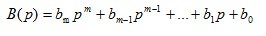 (1.12)
polynomial in the denominator of the transfer function
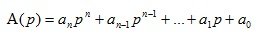 (1.13)
The roots of the equation B (p) = 0 are called zeros of the transfer function . The roots of the equation A (p) = 0 are called the poles of the transfer function .
From the theory of ordinary differential equations with constant coefficients it is known that the equation
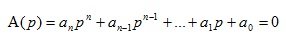 (1.14)
is a characteristic equation of a differential equation
 (1.15)
The roots of the characteristic equation (1.14) allow us to determine the general solution of a homogeneous differential equation
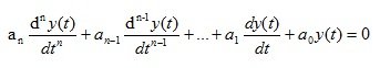 (1.16)
This decision determines the behavior of the automatic system in the absence of external influences, i.e. free movement of the system. Fundamental automatics such as stability and quality of the regulatory process are closely related to the nature of the free movement of the automatic system. Therefore, in the theory of automatic control, great importance is attached to the study of the pole of the transfer function, and the polynomial (1.13) is called the characteristic polynomial of the automatic system.
The transfer function and the structure of a linear stationary system can be represented by an equivalent combination of elementary dynamic links.
Elementary dynamic links (hereinafter referred to as EHL) are called links with the simplest transfer functions not higher than the 2nd order, which cannot be represented as the product of simpler FS.
EHD is depicted in the diagram as a rectangle
System parameters:
k - constant coefficient
T - time period
p - complex variable
? –Damping coefficient (attenuation coefficient)
Typical dynamic links
1. Oscillating link
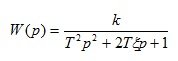 (1.17)
2. Conservative link
 (1.18)
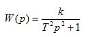
3. Aperiodic (inertial) link 2 order
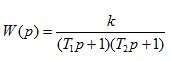 (1.19)
4. Aperiodic (inertial) link 1 order
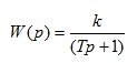 (1.20)
5. Forcing link 1 order
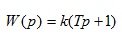 (1.21)
6. Forcing link 2 order
 (1.22)
7. Amplifier (inertia, proportional).
 (1.23)
8. Ideal integrating link
 (1.24)
9. Ideal differentiating link
 (1.25)

Comments
To leave a comment
Mathematical foundations of the theory of automatic control
Terms: Mathematical foundations of the theory of automatic control