Lecture
The frequency characteristics describe the transfer properties of the links (elements) and systems in the steady-state harmonic mode, caused by the external harmonic effect.
The dependence of the ratio of the amplitudes of the output and input signals on the frequency is called the amplitude frequency response (AFC). It is denoted by A (?) (Fig. 5.1).
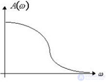
Fig.5.1. Amplitude frequency response
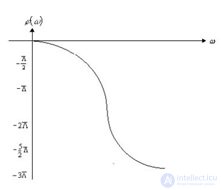
Fig. 5.2. Phase frequency response
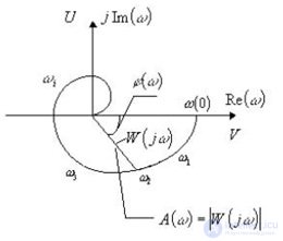
Fig. 5.3. Amplitude and phase response
The dependence of the phase shift on the frequency is called the phase frequency response (phase response), and it is denoted by? (?) (Fig.5.2). The frequency response shows how well the element transmits signals of different frequencies. The phase response shows what kind of lag or advance of the input signal in phase the element creates at different frequencies.
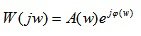
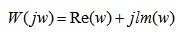
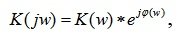
The amplitude frequency and phase frequency characteristics can be combined into one common: amplitude-phase frequency response (AFC) or (AFC) (Fig. 5.3). It is denoted by W (jw) and is a function of a complex variable whose modulus is equal to A (?) , And the argument is equal to? (?).
AFC W (jw), as well as any complex value, can be represented in the exponential:
 (5.1)
(5.1)
or in algebraic form:
 (5.2)
(5.2)
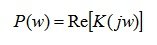
where Re (w) is the projection of the vector W (jw) onto the real axis, and lm (w) is the projection of the vector W (jw) onto the imaginary axis.
Re (w) is called the real frequency response, and lm (w) is the imaginary frequency response.
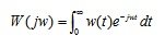
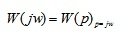
AFH is an Fourier transform image of an impulse transition function:
 (5.3)
(5.3)
The inverse Fourier transform of the AFC will give a pulse transient function:
 (5.4)
(5.4)
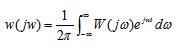
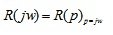
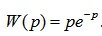
An analytical expression for the AFC of a particular element can be obtained from its transfer function by substituting p = jw:
 (5.5)
(5.5)
The most common is the amplitude-phase frequency response (AFC), which is formally determined from the transfer function by replacing p with the argument jw .
 (5.6)
(5.6)
 (5.7)
(5.7)
 (5.8)
(5.8)
Often W (jw), R (jw), K (jw) is called the complex transfer coefficient.
Amplitude-phase frequency response is a function of the complex variable jw and can be expressed in terms of module and phase. For example, for the AFC link K ( jw ) the module will be K ( jw ) = K ( p ) phase ( p ( w ) = argK ( jw )). AFC can be expressed in the following forms:
- algebraic form:
K ( jw ) = P ( jw ) + jQ ( w ), (5.9)
where P ( jw ) is the real part , jQ ( w ) is the imaginary part;
- indicative form:
 (5.10)
Where:
In equality
 (5.11)
the real part of the complex function K ( jw ), called the real frequency response (VCHH);
 - the imaginary part of the complex function K ( jw ) called imaginary frequency response (MFC).
In equality
 (5.12)
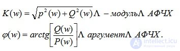
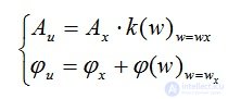
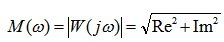
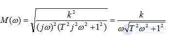
the module of the complex function K ( jw ) is called the amplitude-frequency characteristic (AFC). The amplitude-frequency characteristic of the AFC is the dependence of the system gain on the frequency of the input harmonic signal:
 (5.13)
where Ay ( w ) is the output signal; Ax ( w ) is the input signal.
Therefore, the frequency response is equal to the ratio of the amplitudes of the forced component of the output and input signals.
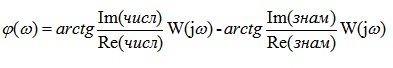
In equality (5.12)  - the argument of the complex function K ( jw ), called the phase frequency response (phase response).
Therefore, the phase response is equal to the phase difference of the forced component of the output and input signals.
The amplitude K ( w ) and phase frequency? (W) characteristics determine the stimulated component of the output signal of the system when it is acted upon by a harmonic input signal specified in a scalar form. So, if the system is affected by the harmonic input signal x (t) of the form, then the forced component of the output signal is determined accordingly. 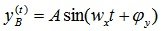 where
where
 (5.14)
The hodograph of the frequency response K ( jw ) is called the trajectory of the point K ( jw ) on the complex plane when the frequency w changes from 0 to? . The hodograph point corresponding to w = 0 is called the beginning of the hodograph, and the point corresponding to w =? end point.
The hodograph is constructed by pairs of real characteristics. P ( w ), Q ( w ) or K ( w ),? (W) .
In practical calculations of ASR, it is convenient to use frequency characteristics constructed in the logarithmic coordinate system (log frequency characteristics — LF). They are characterized by greater linearity and in certain parts of the frequency change can be replaced by straight lines and generally represented by broken lines. Moreover, in most cases, straight line segments can be constructed using some simple rules. In addition, in the logarithmic coordinate system, it is easy to find the characteristics of various compounds of elements, since multiplying and dividing the usual characteristics corresponds to the addition and subtraction of the ordinates of logarithmic characteristics.
The decade is taken as the unit of length on the frequency axis of the LCH. Decade is the frequency interval enclosed between an arbitrary value and its tenfold value. The segment corresponding to one decade is 1.
Usually, logarithmic amplitude frequency response is used in calculations
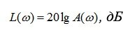 (5.15)
the ordinates of which are measured in logarithmic units - belah or decibels (0.1 bela), abbreviated dB (Fig. 5.4).
Bel is a unit for measuring the power ratio of two signals. If the power of one signal is 10 times more than the power of the other, then these powers differ by 1 B (lg10 = 1).
Because the signal power is proportional to the square of the amplitude, then
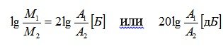
When constructing the phase frequency response, the logarithmic scale is applied only for the abscissa axis.

Fig. 5.4. Logarithmic amplitude-frequency response
Formulas for calculations
 (5.16)
 (5.17)
 (5.18)
 (5.19)
Example 1. The transfer function of an open-loop system is:
 .
.
Determine the frequency response.
Decision:
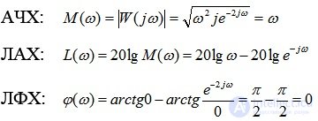
AFH is determined by the formula 5.16:
Frequency response is determined by the formula 5.17:
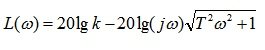
LAH is determined by the formula 5.18:
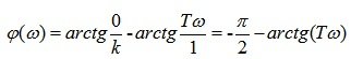
LFH determined by the formula 5.19:
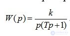
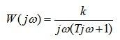
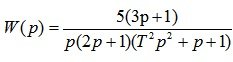
Example 2. The transfer function of the system has the form:
 . Determine the frequency response.
Decision:
AFH: 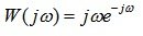
Example 3. Build an LAH graph asymptotically (approximated) for the function
Decision:
System parameters:

Replacing p with jw , we get:
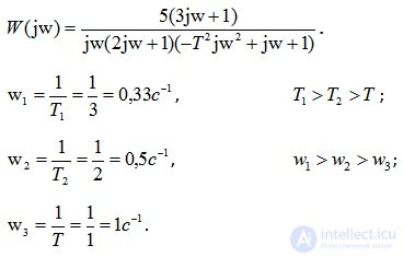
The construction of LAH always starts with an ideally integrating link, which gives a negative slope of the straight line - 20 dB / decade. In the frequency range from w 1 to w 2, the LAH graph will be a straight line with zero slope, since a forcing link (3p + 1) is turned on at this interval, which gives a slope of + 20 dB / decade, which, in combination with the ideal integrating link gives zero angle of the line. In the frequency range from w 2 to w 3, the graph will be a straight line with a negative slope of -20 dB / decade, as the aperiodic link of the 1st order is connected. In the frequency range from w 3 to? the LAH graph will take the form of a straight line with a negative slope of –60 dB / decade, since in this frequency range an oscillating link is connected, giving a negative slope of the straight line –40 dB / decade.
The result of the construction of the LAH is shown in Fig. 5.5.
Fig.5.5. Asymptotic construction of LAH

Comments
To leave a comment
Mathematical foundations of the theory of automatic control
Terms: Mathematical foundations of the theory of automatic control