3.1 The concept of state space and the state-exit model

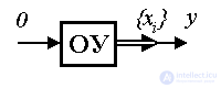
3.1.1. State variables Consider an autonomous dynamic system [M1a] with the output where . Note that for autonomous system solution contains only free component: 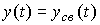. We introduce variables

(3.1) 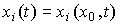, i = 1,2, ... n

with initial values determined by and give the following definition [7] .

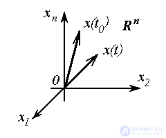
State variables are called linearly independent variables x _i ( t ) such that their values at time t ₀ uniquely determine the state of the system at any time i.e. allow you to find the values ​​of the output variable y ( t ) at arbitrary times t according to the formula

(3.2) .

The procedure for finding the values ​​of a function ( t ) for time points called prediction (see clause 1.1.1). The possibility of prediction is a natural requirement of quality control, which determines the importance of the introduced concept for the nonautonomous (controlled) systems considered below. At the same time, a distinctive feature of state variables is that to predict the behavior of the system at any time t > t ₀ (and control a non-autonomous system) there is enough information about state variables at time t ₀ and no knowledge of the process history is required, i.e. functions x _i ( t ) with t < t _0. The latter serves as the basis for constructing procedures (algorithms) for forecasting and controlling dynamic systems based on the current values ​​of state variables (see § 4.3).

The state variables of an autonomous system can be chosen, in particular, the phase variables of the system, i.e. output variable y ( t ) and n-1 of its derivatives ( t ) . We introduce variables

(3.3) ,

with initial values

(3.4) .

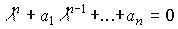
The output of the stationary autonomous system [M1a], i.e. free part of the process = 0, for the case of unequal roots of the characteristic equation, it is determined by the formula (see Section 2.2)

(3.5) ,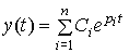

where the coefficients C _i depend on the initial values ​​of the output variable and its derivatives, or taking into account the introduced notation:

(3.6) .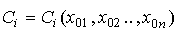

Thus, the behavior of the system under consideration is uniquely determined by the initial values ​​of the variables x _i and, therefore, by definition, these variables are state variables. The total number of state variables is i.e. the order of the differential equation [M1a]. Linear combinations of variables x _i , supplemented to an already selected set, are not state variables, since they lead to a linear dependence of the variables.

Considering the introduced notation, we transform the equation [M1a] to the normal Cauchy form. Differentiating in time the equation (3.5) and substituting the obtained expressions (3.3) and [M1a], we find the so-called equations of state of an autonomous system

(3.7)

The output variable y ( t ) is related to state variables by a trivial expression ( output equation )

(3.8) .

The equations of state (3.7) and output (3.8) are the simplest example of a state-output (CB) model.

Remark 3.1. The choice of dynamic state variables is ambiguous. Not only phase variables can be taken as such variables. 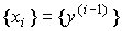, , but also physical variables of the system such as displacement, speed, current, voltage, etc. (see 4.1), as well as any other n linearly independent variables, obtained, for example, as linear combinations of phase and / or physical coordinates.

Naturally, the choice of state variables determines the structure and parameters of the state-output model. In addition to the above method of constructing such a model in the standard form (3.7), (3.8), the CB model can be obtained as a set of models of real physical processes, often corresponding to the elementary links of the first order (see Section 2.3).

3.1.2. State-output and transient models. In the most general case, the equations of state of an autonomous system are presented in the Cauchy normal form, i.e. as a system homogeneous differential equations

[M4a]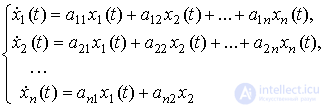

Where , , - constant or time-dependent coefficients (parameters), and the output equation relating the output variable of the system y ( t ) with the variables x _i ( t ) has the form

[M5] ,

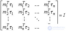
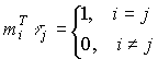
Where - coefficients (parameters). It is easy to show (see below) that the variables x _i ( t ) are indeed state variables and, therefore, the equations [M4a] and [M5] represent the most general state-output model of a linear autonomous dynamic system.

The vector x = x ( t ) of dimension n , whose elements are state variables x _i = x _i ( t ), i.e.

(3.9) = ,

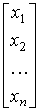called a state vector . The vector x is an element of n - dimensional linear (vector) space. which is called the state space :

The equations [M4a], [M5] can be written in vector-matrix form:

[M6a] ,

[M7] ,

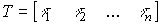
Where , - vector of initial states (initial conditions),

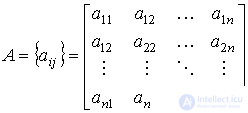- matrix size system , 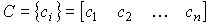- size exit matrix .

In the particular case when the equations of the BC model are presented in the form (3.7) (3.8), we get

, .

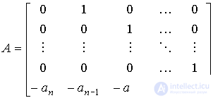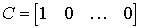By solving a system of differential equations [M4a] with initial conditions called a feature set

(3.10) ,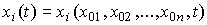

which for t = t ₀ satisfy the initial conditions, and for any - equations [M4a]. Accordingly, the solution of the equation [М6а] will be a vector function

(3.11) .

The solution can be represented as

(3.12) ,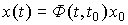

Where - the fundamental (transitional) matrix of the system [М6а]. Substituting (3.12) into the output equation [M7], we obtain the expression for calculating the output variable

(3.13) .

For stationary systems, the transition matrix is

(3.14) .

Putting , we will find:

(3.15)

and

(3.16) .

Remark 3.2. Analysis of equations (3.14) - (3.16) shows the following.

1. Output variable ( t ) at any time uniquely determined by n initial values and therefore by definition the variables really are state variables.

2. Prehistory of the system (its movement at ) does not affect the behavior of the system when .

If for some initial conditions and there is an identity

(3.17) ,

where x * = const, then the value x = x * is called the equilibrium state , or the equilibrium position , of the autonomous system [M6a]. Obviously, in the equilibrium state,

(3.18)

and therefore

(3.19) .

Provided that det A 0, we find that the only equilibrium position of the [M6a] system is the origin of the state space R ⁿ , i.e.

x * = 0,

and with det A = 0, there are nontrivial sets of equilibrium states (straight lines, planes, that is, subspaces that satisfy equation (3.19)).

After substituting x * = 0 into the output equation [M7], we find the equilibrium value of the output variable (see § 2.2.2)

y * = 0.

Formulas (3.14) - (3.16) determine the transient processes of the system - time functions . Graphically, they can be represented as:

• time diagrams (see clause 2.2);
• integral curves.

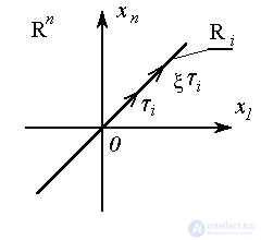
The integral curve (phase trajectory) is a line described by a state vector. in the state space when the variable changes , i.e. hodograph vector functions x ( x ₀ , t   ) by parameter . Phase portrait - a set of phase trajectories corresponding to different values ​​of the initial conditions .

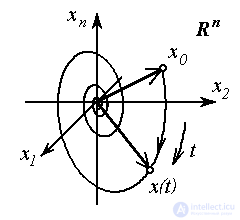
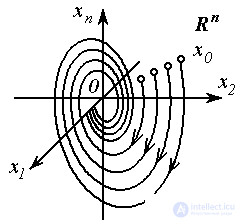
Fig. 3.1. Integral curve in R ⁿ and phase portrait

The concepts introduced above are generalized to the class of multichannel (multiply connected, see § 2.1.3) systems, which are characterized by several output variables y _j , . The general model of a multichannel system includes the equations of state [M4a] and output equations

[M5m]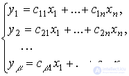

Where - coefficients (parameters).

Define -dimensional vector of outputs

(3.20)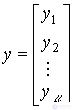

as a vector space of output variables R and write the equation [M5m] in a compact vector-matrix form [M7], i.e.

[M7m] ,

Where - matrix output size . Thus, the state-output model of the multichannel system is represented by the equations [M4], [M5m] or vector-matrix equations [M6a] and [M7m].

3.1.3. Properties of state-exit models . Let us analyze the solutions of the equation of state [M6a], [M7] and the associated transients of the autonomous dynamic system (3.12) - (3.16).

First we define

• eigenvalues ​​(eigenvalues) of the state matrix A as n numbers ;
• characteristic equation

(3.21) ;

• matrix eigenvectors as ,

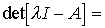
and also (for the case of real eigenvalues ) eigenspaces of the system as sets (straight lines, planes, etc.)

(3.22) ,

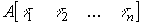
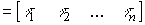
Where - real numbers. Recall that in this case, the eigenvectors satisfy the equations

(3.23) .

Matrix function

(3.24) =

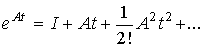
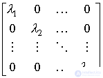
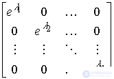
called the matrix exponent. Matrix exponent of the diagonal matrix

;

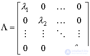calculated by a simple formula

(3.25) .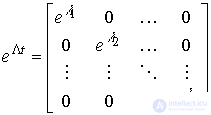

In a more general case (provided ) from the expression (3.23) we obtain:

and therefore matrix A is connected to a diagonal matrix by formula

(3.26) ,

Where

.

Then the matrix exponent is like

(3.27) .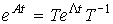

Now, taking into account equation (3.27), we rewrite the formula for calculating the state vector (3.15) as

(3.28) .

Considering that , запишем

and therefore

.

Тогда уравнение (3.28) принимает вид

(3.29) .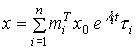

We introduce the notation

(3.30) ( x ₀ )

и запишем формулу (3.29) в виде разложения по собственным векторам

(3.31) ,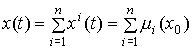

где векторы принадлежат собственным подпространствам системы и называются собственными составляющими решения x ( t ), или модами вектора состояния системы.

Замечание 3.3. Если начальное значение вектора состояния принадлежит собственному подпространству i.e. then

(3.32)

and therefore

(3.33) ,

those. траектория системы целиком лежит в собственном подпространстве R _i .

Такого рода подпространства пространства состояний R ⁿ относятся к классу инвариантных множеств динамической системы.

Проанализируем поведение выходной переменной y ( t ) . Подставляя уравнение ( 3.31 ) в [M7] находим:

(3.34) ,

где y _i ( t ) - моды выходной переменной.

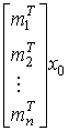
Сравнивая последнее уравнение с выражением (2.20), получим, что неопределенные коэффициенты C _i могут быть рассчитаны как

(3.35) .

Более того,

(3.36) ,

those. полюсы системы p _i совпадают с собственными числами матрицы . Отсюда следует, что совпадают и характеристические уравнения (2.3) и (3.21), или

(3.37) .

Thus, the following properties of state-output models are obtained.

Property 3.1.

.

Property 3.2.

.

Property 3.3.

.

Property 3.4.

.

Property 3.5.

.