Lecture
The superposition operation described in ch. 9, it is often possible to perform more efficiently if, instead of direct processing, processing is carried out using conversion. In fig. 11.2.1, a, b are diagrams for direct execution of the final superposition and discretized superposition. In fig. 11.2.1, g, d are presented the schemes of the superposition operation when the vector  subjected to unitary transformation, the result of which is multiplied by the matrix
  (for the operator of superposition of finite arrays) or matrix
  (for discretized superposition operator). The inverse transform gives the processed vector. According to fig. 11.2.1, a, d, in the case of applying the operator of superposition of finite arrays, the original and processed vectors are related by the following relations:
 (11.2.1а)
and
 . (11.2.1b)
Therefore, the matrix can be represented as a work
 . (11.2.2а)
Similarly
 . (11.2.2b)
To directly perform a superposition of finite arrays, it takes about  operations (here
  - the order of the impulse response matrix). In this case, the fill factor of the matrix
  equals
 . (11.2.3a)
A superposition of discretized arrays requires about  operations, and the fill factor of the matrix
  equals
 . (11.2.3b)
In fig. 11.2.1, e shows a block diagram of cyclic superposition with transformation. In this case, the input vector  serves as the so-called extended input vector, obtained by placing the matrix of the original image
  in the left corner of the square zero matrix
  th order and scan the resulting matrix in columns. Repeating the above reasoning, it can be shown that
 (11.2.4a)
and therefore
 . (11.2.4b)
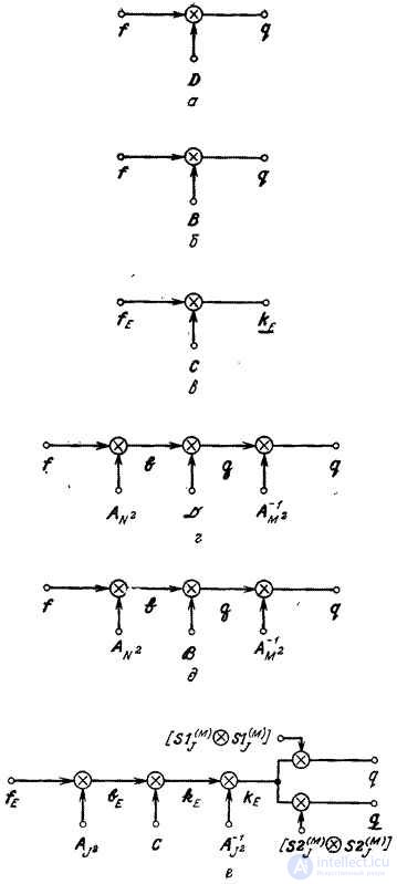
Fig. 11.2.1. Different types of superposition.
a is the final superposition; b - discretized integral superposition; c is a cyclic superposition; g is the final superposition with transformation; e - discretized integral superposition with transformation; e is a cyclic superposition with a transformation.
As noted in ch. 9, for a superposition of finite or discretized arrays, the equivalent output vector can be formed from by choosing specific components of the latter. For superposition of finite arrays
 , (11.2.5а)
and for superposition of discretized arrays
 . (11.2.5b)
With the superposition of finite arrays, the matrix of the processed image is associated with the expanded image matrix  in the following way:
 . (11.2.6a)
When superposing discretized arrays, the matrix of the processed image is equal to
 . (11.2.6b)
The number of arithmetic operations required to calculate the vector  by transformation processing, it can be found from the above formulas, if we put
  :
:
Direct conversion:  .
.
Fast conversion:  .
.
If the matrix  sparse then many of
  multiplications required for filtering operations will not be performed.
From the foregoing, it is easy to conclude that in order to carry out a superposition efficiently, one should choose a transformation that meets two requirements: first, a fast algorithm must exist for it, and, second, the filter matrix of the transformed arrays must be sparse. As an example, we consider the convolution of finite arrays obtained using the Fourier transform [2, 3]. In accordance with Fig. 11.2.1 we set
 , (11.2.7)
Where

at  . Also, assume that the vector
  size
size  represents the extended matrix of the spatially invariant impulse response described by formulas (9.3.2) with
  . Fourier transform from denote by
 . (11.2.8)
The resulting transformation counts are placed on the main diagonal of the size matrix. 
 . (11.2.9)
Using very cumbersome calculations, it can be shown that in the spectral space of the matrix, the convolution operator of finite arrays and the discretized convolution operator can be represented in the following form [4]:
 (11.2.10)
at  and
and
 (11.2.11)
at  where
where
 , (11.2.12а)
 . (11.2.12b)
Thus, both convolution operators in the spectral space contain a matrix of scalar weight factors  and interpolation matrix
  that allows you to associate an input size vector
  with output size vector
  . As a rule, the interpolation matrix
  contains a lot of zero elements, and therefore convolution using the transformation is performed very effectively.
We now consider cyclic convolution performed with the transition to the spectral space. Using arguments similar to the above, it was shown [4] that the filter operator in this case reduces to a scalar operator
 . (11.2.13)
Thus, as can be seen from equalities (11.2.12) and (11.2.13), when convolving in the space of Fourier spectra, the filter matrix can be expressed in a compact closed form. For other unitary transformations, no such expressions were found.
The efficiency of the convolution calculation using the Fourier transform is determined by the fact that the convolution operator  has a cyclic matrix, and the corresponding filter matrix is diagonal. As can be seen from relations (11.1.6), the basic vectors of the Fourier transform are actually the eigenvectors of the matrix [five]. This is not so for a general superposition operation, as well as for a convolution operation using other unitary transformations. However, in many cases the filter matrices
  and
and  contain relatively few non-zero elements, and conversion processing reduces the amount of computation.
In fig. 11.2.2 shows the form of spectra matrices for the three types of the convolution operator for a one-dimensional input vector with a Gaussian impulse response using Fourier and Hadamard transforms [6]. As expected, the transformation coefficient matrices turned out to be significantly more sparse than the original matrices. In addition, it is easy to see that for cyclic convolution with the Fourier transform, the filter matrix is diagonal. In fig. 11.2.3 shows the structure of the matrices of the three convolution operators of two-dimensional signals [4].

Fig. 11.2.2. Matrices of convolution operators of one-dimensional signals using Fourier and Hadamard transforms.
a is the final convolution; b - discretized convolution; c is a cyclic convolution.
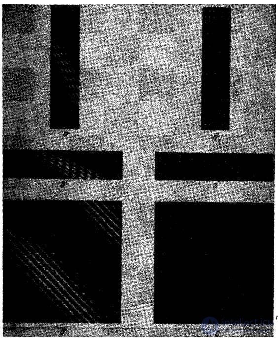
Fig. 11.2.3. Matrices of convolution operators for two-dimensional signals using Fourier transform.
Final convolution: a - directly executed; b - with conversion. Discretized integral convolution: c - directly executed; d - with conversion.
Cyclic convolution: d - directly executed; e - with conversion.

Comments
To leave a comment
Digital image processing
Terms: Digital image processing