6.3. PROCESSING OF QUANTIZED VALUES

Numbers describing images (for example, representing brightness or color coordinates) are usually entered into a digital computer in the form of integer code combinations corresponding to sample quantization levels. Thus, the brightness of a single-color image is usually measured using a linear integer scale bounded by the numbers 0 (black level) and 255 (white level). These integer code combinations, however, should not be construed as arithmetic values. Before processing in the machine, the code combinations should be converted to real decimal numbers corresponding to the quantization level. If this is not done, then you can get completely wrong results. So, if code combinations — level numbers — change non-monotonously along the grayscale, they cannot be used for processing at all. Now consider what happens if these combinations change monotonously and are processed in a digital computer without conversion to decimal numbers - the values ​​of quantization levels.

There are two basic forms of representing numbers in digital computers: as an integer and as a real number. Integers vary from 0 to some maximum value. So, in a 16-bit minicomputer, the largest positive integer is 32,768 ( ). If the result of an arithmetic operation is defined as an integer, and the result is a fractional number, then the fractional part is simply discarded. The ratio of 8/3, for example, will be represented as an integer 2 without decimal point and signs after it. If the processed values ​​are defined as real numbers, then the fractional part of the total of the operation will be saved and contain as many characters as it allows to obtain the capacity of the machine. The ratio of real numbers 8./3. will look like 2.66 ... 66.

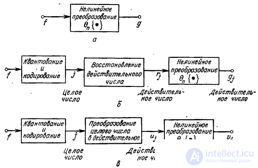
Fig. 6.3.1. Methods for converting quantized signals: a - elementwise transformation of continuous signals; b - conversion of quantized signals represented by real numbers; c - conversion of quantized signals when replacing code combinations with real numbers.

In fig. 6.3.1 for comparison, three methods of signal processing are presented. In fig. 6.3.1, and a continuous scalar varying in the interval subject to conversion resulting in a continuous value

. (6.3.1)

In fig. 6.3.1, b shows the processing scheme in which the scalar value before processing is subjected to uniform quantization and coding. Integer values ​​of code combinations are determined by the formula

, (6.3.2)

where is the symbol , denotes rounding the argument to the nearest integer. Code , defined as an integer, converted to a real number according to the ratio

, (6.3.3а)

or, which is the same,

. (6.3.3b)

Next with a quantized count the necessary operation is performed and a quantized output signal is obtained

, (6.3.4)

different from continuous output , appearing in equality (6.3.1), only because of the quantization error of the initial value.

Unfortunately, often the processing of quantized signals is performed incorrectly - according to the scheme shown in Fig. 6.3.1, c. Code combination considered as an integer, converted to a real number accepting values . After that, according to the formula

(6.3.5)

output values ​​are calculated defined as real numbers. In general has a whole and fractional part. If for example then after the conversion consisting in extracting the square root to the fifth digit, the output signal is obtained . It is clear, of course, that the quantization errors of the input sample will appear in the output countdown . However, there are more serious difficulties, if we assume that can serve as a relatively good approximation of a continuous output signal . Suppose that the number of quantization levels is large enough and therefore

. (6.3.6)

Then the output will be equal to

, (6.3.7)

where are the constants

, (6.3.8a)

. (6.3.8b)

If the conversion linearly then

(6.3.9)

and

. (6.3.10)

Thus, the output signal of the system under consideration (Fig. 6.3.1, c) will be a good approximation of the continuous output signal of a system with analog processing (Fig. 6.3: 1, a) if the conversion performed in the system is linear. On the other hand, if this transformation is non-linear, then the approximation of one signal by another is usually very bad. So, for example, usually the logarithm of a quantized variable differs significantly from the logarithm of a real number formed from a code combination that specifies the number of the quantization level for .