5.4. STATISTICAL DESCRIPTION OF DISCRETE IMAGES

Statistical methods for the description of continuous images given in Ch. 1, can be directly applied to the description of discrete images. In this section, expressions for moments of discrete images are obtained. The joint probability density models are given in the next section.

The average value of the matrix describing a discrete image is a matrix

. (5.4.1)

If this matrix is ​​transformed by columns into a vector, then the average value of this vector is

. (5.4.2)

Correlation of two image elements with coordinates and defined as

. (5.4.3)

The covariance of two elements of the image is

. (5.4.4)

Finally, the dispersion of the image element is

. (5.4.5)

If the image matrix is ​​converted to a vector , the correlation matrix of this vector can be expressed through the correlations of the elements of the matrix :

, (5.4.6a)

or

. (5.4.6b)

Expression

(5.4.7)

is a correlation matrix th and th matrix columns and measures . Consequently, can be represented as a block matrix

(5.4.8)

Covariance matrix of a vector can be obtained on the basis of its correlation matrix and the vector of average values ​​using the ratio

. (5.4.9)

Dispersion matrix array of numbers By definition, it is a matrix whose elements are equal to the variances of the corresponding elements of the array. Matrix elements You can directly select from the matrix blocks :

. (5.4.10)

If a discrete image is represented by an array, stationary in a broad sense, its correlation function can be written as

, (5.4.11)

Where and . Accordingly, the blocks of the covariance matrix (5.4.9) will be connected by the relations

, , (5.4.12а)

, , (5.4.12b)

Where . Thus, for a stationary in a broad sense array

(5.4.13)

The matrix (5.4.13) is block Toeplitz [11]. Finally, if the image correlation function can be written as a product of the correlation functions of rows and columns, then the covariance matrix of the vector representing the image can be written as a direct product of covariance matrices for rows and columns:

(5.4.14)

Where - covariance matrix of matrix columns measuring , but - covariance matrix of matrix rows with sizes .

Consider the case when the covariance matrix of rows of the matrix has the following form:

(5.4.15)

Where - dispersion of image elements. This covariance matrix is ​​an analogue of the continuous autocovariance function of the form - describes the Markov process. In fig. 5.4.1 shows the values ​​of the correlation coefficients of the elements of a typical image line obtained by Davisson [12]. Experimental points are well approximated by the covariance function of a Markov process with a parameter . Similarly, the values ​​of the correlation coefficients in the direction perpendicular to the rows agree well with the Markov covariance function with . If the covariance function can be represented as (5.4.14), then the diagonal correlation coefficients should be equal to the product of the corresponding correlation coefficients along the lines of the image and in the direction perpendicular to them. In this example, it turned out that such an approximation is sufficiently accurate in the range from zero to five discretization steps.

By analogy with the continuous energy spectrum (1.8.11), one can determine the discrete spectral density of a discrete stationary two-dimensional random field representing an image as the result of a two-dimensional discrete Fourier transform of the autocorrelation function of this field. Then, by virtue of equality (5.4.11), we will have

(5.4.16)

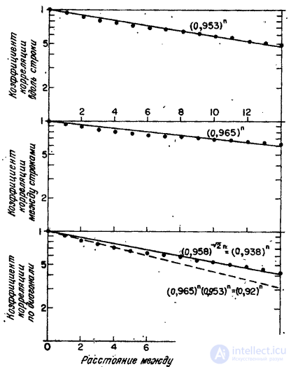
Fig. 5.4.1. An example of correlation dependencies between adjacent image elements.

In fig. 5.4.2 shows the energy spectra of Markov processes.