4.2.1. INFLUENCE OF THE FORM OF DISCRETIZING PULSE

Taking into account the above assumptions, the discretized image can be described by the function

(4.2.1)

where is the sampling function

(4.2.2)

consists of identical pulses forming a grid with spacing . To simplify the notation, the summation limits are chosen symmetrical. We assume that the sampling pulses are normalized so that

(4.2.3)

In the analysis, it can be assumed that the discretization function was obtained by passing a finite set of delta functions through linear filter with impulse response . In this way,

(4.2.4)

Where

(4.2.5)

Substituting expression (4.2.2) into (4.2.1), we obtain the formula for the sampled image

(4.2.6)

The spectrum of this function is

(4.2.7)

Where - the result of the Fourier transform function . The Fourier transform of a finite lattice of discretizing pulses is described by the following relation [5, p. 105]:

(4.2.8)

In fig. 4.2.2 is a graph of the function . With increasing and the right-hand side of formula (4.2.8) in the limit turns into a set of delta functions.

In the image recovery system, a continuous image is obtained by interpolating the samples. Ideal interpolation functions such as and the Bessel [formulas (4.1.14) and (4.1.16)], usually defined on an infinite plane. If the sampling grid has finite dimensions, then the tails of interpolation functions are cut off at the boundaries and errors appear near the edges of the reconstructed image [9, 10]. However, such errors usually become negligible when the distance from the boundaries is 8-10 steps of discretization.

The numerical values ​​of the image samples are obtained by spatial integration. on some final site - the image element. In the scanning system

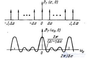
Fig. 4.2.2. Truncated sampling sequence and its spectrum.

(Fig. 4.2.1) integration is actually carried out on the photosensitive surface of the photodetector. The count value corresponding to th element can be found by the formula

(4.2.9)

Where and denote the largest dimensions of this element. Here it is assumed that during the integration time only one sample is taken in the system. Otherwise, you have to solve the complex problem of cross-distortion. In the considered sampling system, the dimensions of the element may be larger than the distance between the samples. Therefore, it is assumed in the model that consecutive (in time) samples correspond to partially overlapping image elements.

By a simple change of variables, equality (4.2.9) can be converted to the form

(4.2.10)

Since it is assumed that only one sample is taken during the integration time, the limits in the integral (4.2.10) can be extended to infinity. In this form, expression (4.2.10) can be considered as the result of convolving the original image with impulse response and subsequent discretization of this convolution in a finite region using delta functions. Then, neglecting the effects associated with the finite sizes of the discretization lattice of the delta functions, we obtain

(4.2.11)

In most sampling systems, the sampling pulse is symmetric, therefore .

The simple form of the relation (4.2.11) is useful in assessing the effects that occur when sampling using pulses of finite width. If the spectrum of the image is limited in width, and if the Nyquist criterion is met, then the finite width of the pulse leads to the same results as if the original image had been subjected to linear distortion (blurring) before perfect sampling. Part 4 will consider methods for compensating for such distortions. However, the finite size of the sampling pulse is not always a disadvantage. Consider the case when the spectrum of the original image is very wide, and therefore it is sampled with insufficient frequency. A finite-sized pulse actually performs low-frequency filtering of the original image, which leads to a narrowing of the spectrum and, therefore, reduces errors caused by the superposition of spectra.