10.2. Fourier transform

The discrete two-dimensional Fourier transform of the matrix of samples of the image is determined [5-10] as a series

, (10.2.1а)

Where and the discrete inverse transform is

. (10.2.1b)

By analogy with the terminology of the continuous Fourier transform, the variables called spatial frequencies. It should be noted that not all researchers use the definition (10.2.1); some prefer to put all the scale constants in the expression for the inverse transformation, while others change the signs in the nuclei to the opposite.

Since the transformation cores are symmetric and separable, the two-dimensional transformation can be performed in the form of successive one-dimensional transformations in rows and columns of the image matrix. The basic functions of the transformation are the exponents with complex indices that can be decomposed into the sine and cosine components. In this way,

, (10.2.2a)

. (10.2.2b)

In fig. 10.2.1 shows the graphs of the sine and cosine components of one-dimensional basis functions of the Fourier transform for . It can be seen that for low frequencies these functions are rough approximations of continuous sinusoids. With increasing frequency, the similarity of basic functions with sinusoids is lost. For the highest frequency, the basis function is a square wave. You can also notice the redundancy of the sets of sinus and cosine components.

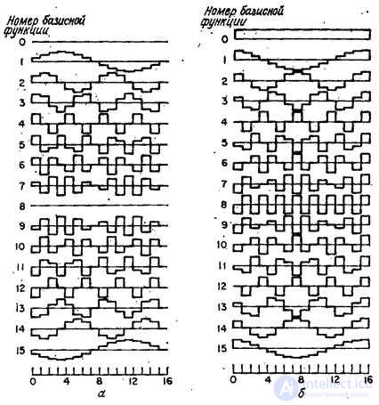
Fig. 10.2.1. Basic functions of the Fourier transform.

and - a sinus (odd) component; b - cosine (even) component.

The image spectrum has many interesting structural features. Spectral component at the origin of the frequency plane

(10.2.3)

equal to increased in times the average (on the original plane) image brightness value. Substituting into equality (10.2.1a)

and where and - permanent, we get

. (10.2.4)

With any integer values and the second exponential factor of equality (10.2.4) turns into unity. Thus, with

, (10.2.5)

which indicates the frequency of the frequency plane. Fig. 10.2.2, and illustrates this result.

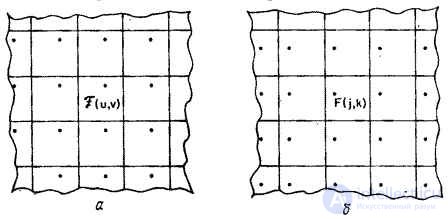
Fig. 10.2.2. Periodic continuation of the image and the Fourier spectrum.

a - spectrum; b - the original image.

The two-dimensional Fourier spectrum of an image is essentially a representation of a two-dimensional field in the form of a Fourier series. In order for such a representation to be fair, the original image must also have a periodic structure, i.e. (as shown in Fig. 10.2.2, b) have a pattern that repeats vertically and horizontally. Thus, the right edge of the image is adjacent to the left, and the top edge - to the bottom. Due to the discontinuities of the brightness values ​​in these places, additional components appear in the image spectrum, lying on the coordinate axes of the frequency plane. These components are not related to the brightness values ​​of the internal points of the image, but they are necessary to reproduce its sharp boundaries.

If the array of samples of the image describes the brightness field, then the numbers will be valid and positive. However, the Fourier spectrum of this image in the general case has complex values. Since the spectrum contains component representing the real and imaginary parts or phase and the modulus of the spectral components for each frequency, it may seem that the Fourier transform increases the dimension of the image. This, however, is not true because has symmetry with respect to complex conjugation. If in equality (10.2.4) we put and equal to integers, then after complex conjugation we get equality

. (10.2.6)

Using substitution and can show that

(10.2.7)

at . Due to the presence of complex conjugate symmetry, almost half of the spectral components turn out to be redundant, i.e. they can be formed from the remaining components. In fig. 10.2.3 areas of the excess spectrum components on the frequency plane are shaded. Of course, harmonics that fall not into the lower, but into the right half-plane can be considered redundant components.

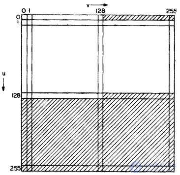
Fig. 10.2.3. Frequency plane.

In fig. 10.2.4 shows photos of the original image and various versions of its Fourier spectrum. Since the dynamic range of the spectral components is much wider than the linear portion of the exposure interval of the film, the spectra must be compressed. Dynamic range compression can be accomplished by limiting large spectral components or logarithmic transformation of all components of the spectrum according to the relation

, (10.2.8)

Where and - scale constants. In fig. 10.2.4, b are given (on a logarithmic scale with and ) moduli of harmonics of the spectrum, calculated in accordance with the equality (10.2.1a). In fig. 10.2.4, the same spectrum is shown, in which the highest harmonics, constituting 25% of all components of the spectrum, were limited in magnitude. In the mathematical analysis of continuous signals, the origin of the frequency plane is usually placed in its geometric center. Similarly, in the diffraction pattern obtained using a coherent optical system for a transparency with a transmittance , the harmonic with zero frequency appears in the center. The two-dimensional discrete Fourier spectrum found with the help of a computer can be changed by simply rearranging the coefficients so that the origin of the coordinates also appears in the center of the array. The same result can be obtained differently if the image samples are previously multiplied by the coefficients of the form . Then the quadrants of the spectrum, calculated according to the formula (10.2.1a), are automatically swapped during the calculation. This statement can be proved by using the relation (10.2.4), putting in it . Then by virtue of identity

(10.2.9)

expression (10.2.4) can be written in the following form:

. (10.2.10)

In fig. 10.2.4, g is the spectrum with permuted harmonics.

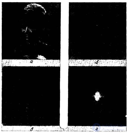
Fig. 10.2.4. Fourier transform image "Portrait".

a - the original image; b - modules of harmonics of the spectrum (on a logarithmic scale, without rearrangement of harmonics); c — spectrum with limited largest harmonics (without their rearrangement); (d) spectrum with limited greatest harmonics (after their rearrangement).

The direct and inverse Fourier transforms (10.2.1) can be represented in vector form

, (10.2.11a)

but

, (10.2.11b)

Where and - vectors obtained respectively by scanning the columns of matrices and . Since the transformation matrix can be written as a direct work

(10.2.12)

Where

, (10.2.13)

, then the image and spectrum matrices are related by

(10.2.14a)

and

. (10.2.14b)

It is clear that the properties of the Fourier transform established for the series (10.2.1) are also preserved during its matrix recording.

Although the Fourier transform has many useful properties for analyzing, it has two significant drawbacks: first, all calculations have to be made not with real, but with complex numbers, and, second, the series converge slowly. The last remark, which is very important for image coding problems, can be explained by rewriting the definition (10.2.1b) in the following form:

, (10.2.15)

Where - low-frequency region of the frequency plane, which is shown in Fig. 10.2.5 shaded. If the upper bound and fixed and image size is relatively small, the value enclosed in square brackets can be very different from , until and won't get big enough. In the future, the issue of convergence of transformations will be analyzed from a quantitative standpoint. Qualitatively, it can be pointed out that the poor convergence of the Fourier transform is due to image jumps that occur on the transition lines from the left edge of the image to the right and from the top to the bottom. These gaps lead to the appearance of large components in the spectrum with high spatial frequencies.

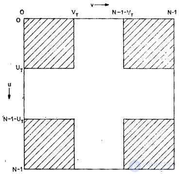
Fig. 10.2.5. Low frequency region of the frequency plane.