9.2. DISCRETED SUPERPOSITION OPERATOR

In digital image processing, in many cases it is required to convert the integral superposition operator in discrete form, connecting continuous images at the input and output of the linear system. Phenomena such as image blurring caused by imperfections in the optical system, aperture distortion or distortion when viewed through a turbulent atmosphere can be described using the following integral equation:

, (9.2.1а)

Where and describe the input and output images, respectively, and the core represents the impulse response of a linear system. The impulse response can be a function of four variables — the coordinates of the points of the input and output planes. If the linear system is spatially invariant, then the image at its output can be described using the convolution integral

. (9.2.1b)

With discrete processing, the output image will be represented by samples. Therefore, the integral of superposition or convolution should be transformed so as to express explicitly the connection of the output image samples with the values ​​of the function describing the input image. The question of the discrete representation of integral transforms is important, since the resulting errors can lead to large errors in the processed image or even to the loss of stability of the digital processing process. In addition, the choice of the discrete-representation algorithm, as a rule, greatly depends on the complexity of the processing itself.

In the first stage of the discretization process of the superposition integral, the output image is discretized using a lattice from Dirac delta pulses separated by an interval . The result is an array of samples.

, (9.2.2)

Where . The delta function can be introduced into the integrand of the integral (9.2.1a); the result is a ratio

. (9.2.3)

It should be noted that the output image is discretized according to the coordinates of the plane of the observed image. and does not affect current variables on which integration is carried out.

In the next step, the impulse response should be limited in duration. For this we set

(9.2.4)

at and . Then

. (9.2.5)

It should be noted that the truncation of the impulse response is equivalent to multiplying it by the weighting function (“window”) equal to one inside the square , and zero beyond. According to the convolution spectrum theorem, the spectrum obtained after truncating an image is equal to the convolution of the image spectra and weight function (window) and the spectrum of the latter is a two-dimensional sinc function. Such a distortion of the spectrum leads to the appearance of parasitic components with high spatial frequencies, grouped near frequencies that are multiple (the Gibbs phenomenon). The distortion of the truncation can be reduced by using more sophisticated weight functions, such as Bartlett, Blackman, Hamming, or Hann's windows [3], which can smooth out unwanted effects associated with the presence of gaps in a rectangular window. The choice of a suitable window is of great importance, since the incorrectness of the integral transform (9.2.1a) can lead to a sharp increase in distortion caused by the truncation of the impulse response in the image reconstruction process.

The next step in the sampling process is that the continuous source image represented by a set of values ​​describing its function in nodes of a rectangular grid with a step and size . This operation is not a sampling of real samples, but only a mathematical transformation, which results in an array

, (9.2.6)

Where , and and denote the minimum and maximum index values .

If the ultimate goal is to estimate the continuous source image by processing real samples of the observed physical field, then step must be taken small enough for the Nyquist criterion to be satisfied for the original image. This means that if the original image has a spectrum of finite width, then the distance between the nodes should be set equal to the corresponding Nyquist interval. Ideally, this provides the ability to accurately restore the image. by interpolating estimated values .

Using the formulas for the approximate calculation of integrals, in equality (9.2.5), the integral can be approximated by a sum [2]. In this case, the actual image samples can be described by the expression

, (9.2.7)

Where - weight coefficients in a particular approximate formula used for calculations. Usually they use the formula of rectangles, for which all weights are equal to one. In any case, it is convenient to combine the weights and impulse response counts, so that

. (9.2.8)

Then

. (9.2.9)

It should be noted that the function has not been sampled by the first two variables. In the formulas, its values ​​simply appear in the corresponding points. The limits of summation in equality (9.2.9) are equal

, (9.2.10)

where is the symbol denotes rounding to the nearest integer.

In fig. 9.2.1 is an example of how real counts output image is mapped to anchor points source image. In this example, the interval between the nodes is twice as large as the distance between the actual samples. The impulse response values ​​used in calculating the sum (9.2.9) are shown in dots in this figure.

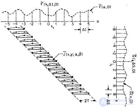
Fig. 9.2.1. The relationship between the real image samples and the values ​​of the original image at the nodal points in the numerical representation of the superposition integral.

In connection with the discrete representation (9.2.9) of a linear integral transform, an important note should be made: regardless of the ratio between the number of nodal points and the number of real samples, the area of ​​the original image where the nodal points that affect the values ​​of real samples are located, always turns out to be larger than the area of ​​the sampled output image . As shown in fig. 9.2.2, the sizes of both images with an accuracy of one sampling interval are related by the relation

. (9.2.11)

Fig. 9.2.2. The ratio between the regions of the location of real samples and nodal points in the numerical representation of the integral of the superposition.

A - the original image; B - area of ​​location of counts of the observed image; In - the location of the nodal points.

So, a discrete finite model of a linear integral transform was built, which links the output image samples with the values ​​of the elements of the original image through the mathematical operation of a discrete linear transformation. Such an operation is an approximation of the continuous transform, since the impulse response subjected to truncation, and the integral was calculated by approximate quadrature formulas. It is clear that, by expanding the domain of the impulse response, the truncation error can be made arbitrarily small, although this is associated with an increase in the amount of computation. Errors due to the approximate calculation of the integrals can be reduced by applying more accurate quadrature formulas, but also at the cost of complicating the calculations. It should be noted, however, that the discrete version of the linear integral transform is an exact approximation of the latter, if all the functions of the spatial variables included in formula (9.2.1) have spectra of limited width, and the intervals when sampling the output image and the numerical representation of the original image are selected in according to the Nyquist criterion [4]. The question of the accuracy and stability of the discrete representation is considered in Chapter. 14.

It often turns out that it is more convenient to use relation (9.2.9) if it is represented in a vector form. To this end, the numbering of the elements of the arrays and should be changed so that arrays of sizes are formed respectively and with positive indices. Assume that

, (9.2.12а)

Where , but

, (9.2.12b)

Where . In addition, we define the impulse response so that

. (9.2.12c)

In fig. 9.2.3 shows the geometric relationships between these functions.

Fig. 9.2.3. Arrays of samples of the image and impulse response.

The discrete transformation (9.2.9) with respect to shifted arrays has the following form:

, (9.2.13)

Where a

.

Using the methodology described in Ch. 5, vectors can be formed and which are the scan matrix and by columns. These vectors are related by the relation [1]

(9.2.14)

Where - size matrix having the following structure:

. (9.2.15)

Matrix elements determined by equality

(9.2.16)

at , where there is an odd integer closest to the size of the impulse response, expressed by the number of discretization steps . Further, for simplicity, the matrix will be called the lubrication matrix. If the impulse response is invariant with respect to the bias, i.e.

, (9.2.17)

then the operation of discrete superposition (9.2.13) turns into a discrete convolution:

. (9.2.18)

An interesting case when where - integer. Wherein

(9.2.19)

Now the elements of the blur matrix are equal

, (9.2.20)

Where and . Further, if , the elements of the blur matrix take the form

. (9.2.21)

Besides,

. (9.2.22)

Therefore, all rows of the matrix are obtained by shifting the first row. Then the operator is a discretized convolution operator, and the sum representation (9.2.19) is simplified:

. (9.2.23)

In fig. 9.2.4, and the printout of matrices of the discretized convolution operator is given, when the input array consists of counts impulse response is presented counts and the output array contains countdown . In fig. 9.2.4, b shows the view of the matrix for the case of higher dimensions when and the impulse response is Gaussian.

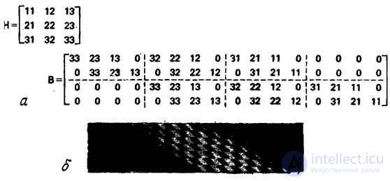
Fig. 9.2.4. Examples of matrices of discretized convolution operators.

a - the general case ; b - impulse response of the Gaussian form, .

Assume that the impulse response is spatially invariant and separable, i.e.

, (9.2.24)

where are the matrices and size have the following structure:

. (9.2.25)

In this case, the calculation of a two-dimensional convolution is reduced to the sequential execution of convolutions in rows and columns of the matrix of the original image. In this way,

. (9.2.26)

To perform a superposition operation or to calculate a convolution in vector form arithmetic operations, and this number does not include multiplication by zero elements of the matrix . If we separate the convolution operator, then for calculations in the matrix form it suffices arithmetic operations.

Suppose that with the same impulse response size to an array of image size counts To simulate the process of continuous superposition, a superposition operator of finite arrays and a discretized superposition operator are applied. Then the array processed by the first operator coincides with the array obtained as a result of the action of the second operator, which is surrounded by a strip of extra elements, and vice versa, if the sizes of the processed arrays are the same, then the border elements of the array obtained with the help of the finite superposition operator will be distorted. Thus, one should carefully use the operator of a superposition of finite arrays to simulate continuous processes.