Lecture
It is known that the Fourier series for any continuous real and symmetric (even) function contains only real coefficients corresponding to the cosine terms of the series. In appropriate interpretation, this result can be extended to the discrete Fourier transform of images. There are [11] two methods for obtaining symmetric images (Fig. 10.3.1). According to the first of them, its mirror reflections are closely attached to the image. According to the second method, the original and reflections are attached, imposing extreme elements. So from the original array containing  elements, in the first case (called the even cosine transform), we get an array of
  elements, and in the second case (called the odd cosine transform), an array of
  items.
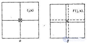
Fig. 10.3.1. Construction of a symmetric image intended for the cosine transform.
a - reflection relative to the edge: b - reflection relative to the extreme elements.
Even symmetric cosine transform
Assume that a symmetric array is formed by mirroring the original array relative to its edges according to the relation
 (10.3.1)
Thus constructed array  symmetric about the point
  ,
,  . Having calculated the Fourier transform for the case when the origin is at the center of symmetry, we get
 , (10.3.2)
Where  . Since the array is symmetric and consists of real numbers, the relation (10.3.2) can be reduced to the form
 . (10.3.3)
On the other hand, the spectral components of the form (10.3.3) can be found by calculating the Fourier transform of the array  by
by  points:
 . (10.3.4)
The direct even cosine transform by definition [12] is equal to the sum (10.3.3) multiplied by the normalizing factor, i.e.
 , (10.3.5a)
and the inverse transform is determined by
 , (10.3.5b)
Where  , but
, but  at
at  . It turned out that the basis functions of the even cosine transform belong to the class of discrete Chebyshev polynomials [12].
In fig. 10.3.2 shows the graphs of the basis functions of an even symmetric cosine transform at  . Samples of the spectrum obtained with an even symmetric cosine transform are shown in Fig. 10.3.3. The origin of coordinates is located in the upper left corner of each image, which is consistent with the order adopted in matrix theory. It should be noted that here, as in the case of the Fourier transform, the main part of the image energy is concentrated in the region of low spatial frequencies.
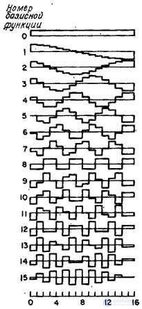
Fig. 10.3.2. Basic functions of the cosine transform.
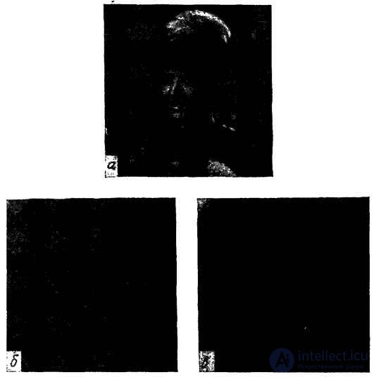
Fig. 10.3.3. Cosine transformation of the image "Portrait".
a - original image: b - cosine spectrum in a logarithmic scale along the amplitude axis; c - spectrum with limited greatest harmonics.
Odd symmetric cosine transform
In the case of an odd cosine transform, the structure of a symmetric array is defined as follows:
 (10.3.6)
Calculating a two-dimensional Fourier transform from such an array gives
 , (10.3.7)
Where  . Since the Fourier transform has a symmetry property with respect to complex conjugation, for real images
 . (10.3.8)
Consequently,  it is enough to calculate only for nonnegative values of the indices
  . Also, since the function takes real values and is symmetric, then also has valid values. Thus, the ratio (10.3.2) can be represented as follows:
 , (10.3.9)
where is the array  obtained from the image matrix weighing its elements in accordance with the formula
 (10.3.10)
The odd cosine transform is simply the normalized version of equality (10.3.9), and the normalization is carried out so that the basis functions become orthonormal. Thus, the odd cosine transform is determined by the ratios
 at
at  , (10.3.11a)
 at
at  . (10.3.11b)
Same transformation
 at
at  , (10.3.12а)
 at
at  (10.3.12b)
gives a matrix of weighted samples . Then the original array can be restored using the formula
 (10.3.13)
The basis functions of the odd cosine transform are separable, so that two-dimensional odd cosine transform can be performed using successive one-dimensional transforms. In addition, the odd cosine transform can be found using the Fourier transform algorithm with an odd number of elements, since
 . (10.3.14)

Comments
To leave a comment
Digital image processing
Terms: Digital image processing