5.5. MODELS OF DENSITY OF PROBABILITY OF DISCRETE IMAGES

Discrete image represented by an array can be fully described using the joint probability density of its elements. When specified in matrix form, this density is written as

, (5.5.1а)

and in vector form - as

, (5.5.1b)

Where determines the order of joint density. If all elements of the image are statistically independent, then the joint probability density is equal to the product of one-dimensional unconditional densities.

. (5.5.2)

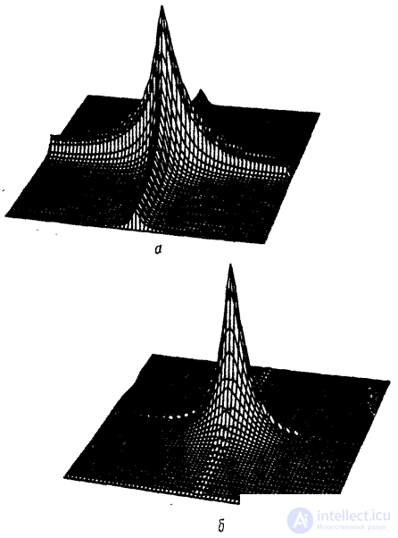
Fig. 5.4.2. Energy spectra of Markov image-modeling processes ( , on the vertical axis, the logarithmic scale): a is a separable spectrum; b - spectrum with circular symmetry.

The most common type of joint probability density is gaussian density.

, (5.5.3)

Where - vector covariance matrix , - average value and the symbol marked matrix determinant . The Gaussian density is a useful model of the joint probability density of the coefficients obtained as a result of unitary transformations of images. However, the Gaussian density is not suitable for describing the brightness of image elements, since the brightness can only be positive, and Gaussian random variables take both positive and negative values.

Expressions for joint densities that are not Gaussian are rarely found in the literature. Huns [13] developed a method for forming such high order densities based on a given unconditional first-order density and a given covariance matrix of ensemble elements. For zero-mean density, this procedure reduces to a linear transformation of a set of independent random variables. whose joint probability density is

(5.5.4)

can be written as a product of given first-order densities. Then the desired joint probability density is

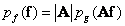, (5.5.5)

Where

, (5.5.6)

but denotes the determinant of the matrix . Matrix columns are eigenvectors of a given covariance matrix and matrix - diagonal and consists of the eigenvalues ​​of this matrix, and the relation

. (5.5.7)

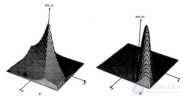
Fig. 5.5.1. Two-dimensional probability density pairs of correlated random variables : a - probability density distribution of Laplace; b - Rayleigh probability distribution density.

In fig. 5.5.1 shows two-dimensional probability densities of a pair of correlated random variables, the unconditional distributions of which are Rayleigh or Laplace distributions. The multidimensional model with the Rayleigh distribution is useful in considering the joint probability density of the brightness of the image elements, and the model with the Laplace distribution is used to statistically describe the sequence of difference signals generated in the image coding systems using the prediction method.

The next chapter discusses the quantization technique, that is, the representation of samples using a discrete set of numbers, called quantization levels. Let be denotes level of quantization for the image element that occupies -e place in the vector image . Then the probability of obtaining one of the possible values ​​of the vector can be expressed through the joint distribution of probabilities of sample values ​​as follows:

, (5.5.8)

Where . Usually for all components of the vector choose the same set of quantization levels and the joint probability distribution takes the form

. (5.5.9)

The probability distributions of sample values ​​can be estimated by measuring the corresponding frequencies. So, one-dimensional distribution vector components

(5.5.10)

can be estimated by analyzing a large set of images belonging to the same class, such as fluorograms, aerial photographs of fields, etc. The estimate of the one-dimensional probability distribution is the distribution of relative frequencies

, (5.5.11)

Where - the total number of images studied, and - number of shots for which , . If the source of images is stationary, then one-dimensional distributions (5.5.10) will be the same for all components of the vector, i.e. they will not depend on . In addition, if the source of images is ergodic, then ensemble averaging (measurements using a set of images) can be replaced by averaging over spatial coordinates. If the ergodicity assumption is true, then the one-dimensional distribution can be estimated from the frequencies

, (5.5.12)

Where - the number of elements of the investigated image, for which , and , but .

In fig. 5.5.2 shows one-dimensional histograms of red, green and blue coordinates of the color of the color image "Portrait". In most natural images, dark elements are much larger than light ones, and the frequencies decrease with an increase in brightness approximately exponentially.

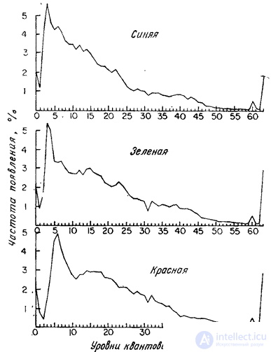
Fig. 5.5.2. Typical histograms of red, green and blue color image color coordinates.

An estimate of the two-dimensional probability distribution for an ergodic source of images can be found using a second-order frequency distribution, which is obtained by counting the cases of the occurrence of certain pairs of element values ​​separated by a given distance. Assume that and there are two image elements separated by a length which is tilted to the horizontal axis at an angle (fig. 5.5.3). Since the elements form a rectangular lattice, the parameters , may take only some discrete values. The relative frequency of the second order is

, (5.5.13)

Where - the number of pairs of picture elements for which and . Denominator of a fraction (5.5.13) represents the total number of pairs of elements that are separated by segments with the same parameters . Due to edge effects .

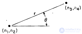
Fig. 5.5.3. Mutual arrangement of a pair of image elements.

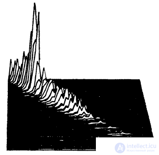
Fig. 5.5.4. Second-order histograms for the “Portrait” image.

The second-order histograms for the “Portrait” image are presented in Fig.5.5.4. The elements of the image with the increase in the distance between them become less correlated, and the frequencies are distributed on the plane more evenly.