Chapter 6. QUANTIZATION OF IMAGES

Any analog value to be processed in a digital computer or digital system must be represented as an integer number proportional to the value of this value. The process of converting samples with a continuous set of values ​​into samples with discrete values ​​is called quantization. The next two sections give a mathematical analysis of the quantization process, which is valid not only for images, but in general for a wide class of signals that one has to face in image processing systems. Then the processing of quantized samples is considered. The last two sections describe the subjective effects that occur when quantizing single-color and color images.

6.1. QUANTIZATION OF SCALAR VALUES

Fig. 6.1.1 illustrates a typical example of scalar quantization. In the quantization process, the sample value of the analog signal is compared with a set of threshold levels. If the sample falls in the interval between two adjacent threshold levels, then the value of the fixed quantization level corresponding to the given interval is attributed to it. In a digital system, a binary code combination is assigned to each quantized sample. In this example, a uniform code is applied having a constant length of code combinations.

Starting a quantitative analysis of quantization of scalar quantities, we assume that and denote, respectively, the values ​​of the reference of the actual scalar signal before and after quantization. It is assumed that - random variable with probability density . In addition, it is assumed that does not go beyond a certain interval:

, (6.1.1)

Where and - upper and lower limits of the interval.

When solving the quantization problem, it is necessary to choose such a set of threshold levels. and quantization levels , what if

, (6.1.2)

then the original count is replaced by a number equal to the quantization level . In fig. 6.1.2, and an example is given of the arrangement of threshold levels and quantization levels on a segment of the numerical axis containing threshold levels. Another common form of representing the characteristics of a quantizer is a step curve (Fig. 6.1.2, b).

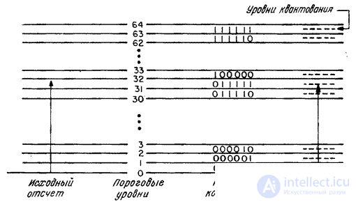
Fig. 6.1.1. An example of signal quantization.

The quantization levels and threshold levels are chosen so as to minimize to a minimum some given value characterizing the quantization error, i.e. the degree of difference between and . As a measure of quantization error, a rms error is usually chosen. If a - the number of quantization levels, then the root-mean-square quantization error is

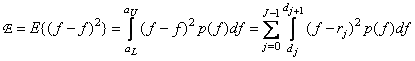. (6.1.3)

If the number large, then the probability density of the values ​​of the quantized signal at each of the intervals can be considered constant and equal . Consequently,

(6.1.4)

or after calculating the integrals

(6.1.5)

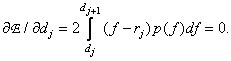
Optimal quantization level position in the interval can be found by solving the problem of the minimum error as functions . Equating zero derivative

, (6.1.6)

we get

. (6.1.7)

Thus, under the assumptions made, the optimal position of the quantization level is the midpoint of the interval between adjacent threshold levels.

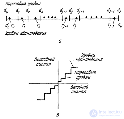
Fig. 6.1.2. Thresholds and quantization levels.

Substituting the corresponding values ​​in the expression for the quantization error, we get

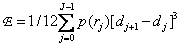. (6.1.8)

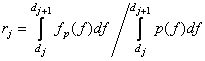
The optimal position of the threshold levels can be determined by finding the minimum error Lagrange multipliers. Using this method, Panther and Data [1] showed that the positions of threshold levels are fairly accurately determined by the formula

(6.1.9a)

Where

, (6.1.9b)

but . If the probability density of sample values ​​is uniform, then the threshold levels will be spaced evenly. With non-uniform densities, threshold levels are more common in those areas where the probability density is high, and less often where it is low. For most types of probability density, which are usually used in image description, integrals (6.1.9) cannot be taken, and the position of threshold levels has to be found using numerical integration.

If the number of quantization levels is small, then the approximation by which equality (6.1.4) is obtained becomes unjustified and the exact expression for the error (6.1.3) should be used. Differentiating it by variables and and equating the derivatives to zero, we get

(6.1.10a)

(6.1.10b)

After transformations we come to the system of equations

(6.1.11a)

. (6.1.11b)

Solving these equations in a recurrent way, it is possible for a given probability density find the optimal values ​​of threshold levels and quantization levels. Max [2] solved this problem for Gaussian density and compiled tables of optimal placement of threshold levels depending on the number of quantization levels. In tab. 6.1.1 shows the location of the quantization levels and threshold levels in the Max quantizer for the densities of the Gauss, Laplace, Rayleigh, and uniform probability distributions.

Table 6.1.1. The location of the quantization levels and threshold levels in the Max quantizer

It is easy to show that if the threshold levels and quantization levels are chosen according to equality (6.1.11), then the root-mean-square quantization error decreases to

(6.1.12a)

or in shorter form

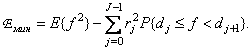(6.1.12b)

For the particular case of the density of the uniform probability distribution, the minimum root mean square error is equal to

(6.1.13)

For most other types of probability density, quantization error has to be determined by calculations.

Uneven quantization can be reduced to a uniform using a nonlinear transformation, as shown in Fig. 6.1.3. The counting is subjected to nonlinear transformation, will be evenly quantized and subjected to the inverse nonlinear transformation [3]. In quantization systems with transformation, they strive to make the probability density of the transformed samples at the input of the quantizer uniform. The converted count (Fig. 6.1.3) is

, (6.1.14)

moreover, nonlinear transformation chosen such that the probability density turns out to be uniform, i.e.

. (6.1.15)

in the interval . If a - a random value with zero mean, then the desired characteristic of the nonlinear element has the form [4]

. (6.1.16)

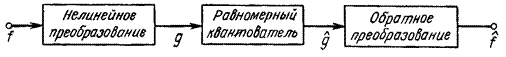
Fig. 6.1.3. Quantizer with compression.

Table 6.1.2. Transformation quantization

Probability density	Direct conversion	Inverse transform
Gaussian Rayleigh Laplace

Thus, it coincides with the probability distribution function of a quantity. In tab. 6.1.2 shows the characteristics of direct and inverse nonlinear transformations for the densities of the probability distributions of Gauss, Rayleigh, Laplace.