4.1.2. DISCRETIZATION OF RANDOM IMAGES

Above, when analyzing questions about discretization and reconstruction, images it was assumed that the function describing the original image is deterministic. It was shown that if this image has a spectrum of limited width, then the set of image samples taken at the Nyquist frequency at discrete points is sufficient to reconstruct an exact copy of the original image from samples. A similar conclusion holds in the case of discretization of random two-dimensional fields. Let be denotes a continuous two-dimensional stationary random process with known mean values and autocorrelation function

(4.1.17)

Where and . Using a set of delta functions, we will discretize this process. As a result, we get

(4.1.18)

The autocorrelation function of the discretized process is

(4.1.19)

The first factor of the right side of this equality is the autocorrelation function of the stationary source image. It should be noted that the product on the right-hand side of equality (4.1.19) of two discretizing delta functions is a delta function of the form

(4.1.20)

Consequently, the discretized random field representing the image is also stationary and has an autocorrelation function.

(4.1.21)

Using the two-dimensional Fourier transform of the autocorrelation function (4.1.21), we find the energy spectrum of a discretized random field. According to the spectrum theorem,

(4.1.22)

Where and designate, respectively, the spectral density of the original and discretized images, and - the result of the Fourier transform of the sampling delta functions. Further, repeating the steps taken in deriving the relation (4.1.7), we obtain that the energy spectrum of the discretized image can be written in the following form:

(4.1.23)

Thus, the energy spectrum of the sampled image is formed by repetition of the energy spectrum of the continuous source image in the spatial frequency domain at intervals that are multiples of the spatial sampling frequency . If the width of the energy spectrum of the continuous image is limited so that at and Where and - boundary frequencies, then in the sum (4.1.23) the individual spectra will not overlap in the case when the sampling intervals satisfy the conditions and . Continuous random image can be recovered from samples of the original random image using interpolation using the formula

(4.1.24)

Where - deterministic interpolation function. It can be achieved that the reconstructed field and the original image are equivalent in the mean square sense [5, p. 284], i.e.

(4.1.25)

For this, it suffices that the Nyquist criterion is satisfied and a sufficiently “good” function was chosen as an interpolation function, such as, for example, the Bessel or , defined by the formulas (4.1.16) and (4.1.14).

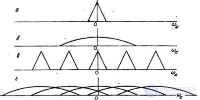
Fig. 4.1.4. Spectra of a discretized image containing signal and interference.

a - signal: b - interference; в - sampled signal; g - discrete interference.

The results can be directly applied to the practical problem of discretization of the sum of the deterministic image and additive noise, the model of which is a random field. In fig. 4.1.4 shows an example of the energy spectrum of a discretized noisy image. This example indicates the possibility of serious difficulties. The noise spectrum may be wider than the spectrum of the useful image, and if the noise is sampled with insufficient frequency, then the "tails" of the noise spectrum will fall into the passband of the recovery filter. This will increase the distortion caused by noise. To eliminate this difficulty, before sampling, you should, of course, filter the noisy image in order to narrow the noise spectrum.