11.3. Convolution using FFT

As already noted, for the convolution operator of finite arrays or the discretized convolution operator, the equivalent output vector can be found by choosing certain elements of the extended output cyclic convolution vector or its corresponding matrix . This situation in combination with equality (11.2.13) leads to a very efficient procedure for calculating convolution, consisting of the following steps:

1. Write the impulse response matrix in the upper left corner of the zero matrix. th order, and for the case of convolution of finite arrays and for discretized convolution. Perform a two-dimensional Fourier transform of the extended impulse response matrix.

. (11.3.1)

2. Write the matrix of the original image in the upper left corner of the zero matrix -th order and perform a two-dimensional Fourier transform of the augmented matrix of the original image

. (11.3.2)

3. Perform scalar multiplication

, (11.3.3)

Where and .

4. Perform inverse Fourier transform

. (11.3.4)

5. After selecting the desired elements to form the desired output matrix

(11.3.5a)

or

. (11.3.5b)

It is important that order extended matrices and satisfied the corresponding inequalities. With on the left and top edges of the output matrix there will be bands of erroneous elements having a width of the countdown (fig. 11.3.1, a, b). They are formed as a result of the so-called cyclic error associated with the incorrect application of the FFT method to calculate convolution. In addition, when performing convolution of finite arrays ( -convolution) will be lost elements of the output array, arranged by stripes in the right and lower parts of it. If we put then at - The output matrix will be completely filled with the correct readings. To calculate -convolution with , it is necessary to cut off the right and bottom edges of the original matrix. However, the result is that the elements of the output array, located on the top and on the left, will be erroneous.

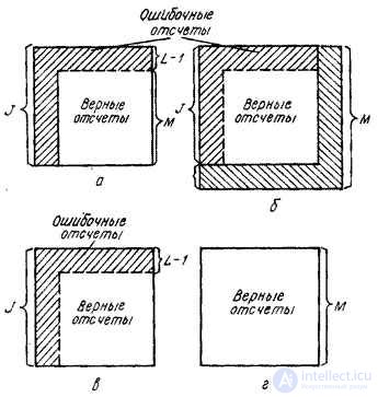
Fig. 11.3.1. Cyclic errors. (Bottom and right sides of the matrix cut off.)

a - type filtering ; .

b - type filtering ; .

c - type filtering ; .

g - type filtering ; .

In signal processing, in many cases, it turns out that different input arrays are affected by operators with the same impulse response and, consequently, the first stage of the algorithm (calculation ) enough to run only once. When using the FFT algorithm for the cases of direct and inverse transformations, it is required to perform approximately arithmetic operations. Scalar multiplication is done for operations, i.e., everything is required operations. If the input matrix contains items, output and impulse response matrix elements, then to calculate the final convolution is required operations, and for discretized convolution operations. If size impulse response matrices are large enough compared to the size the original matrix, the convolution with the transformation turns out to be more efficient than the direct convolution, and the number of operations can be reduced ten times or more. In fig. 11.3.2 shows the graph of dependence from for the case when both methods for calculating the convolution of finite arrays (direct and with Fourier transform) have the same efficiency. The jaggedness of the graphics is due to the fact that with increasing parameter changes in steps, taking values ​​64, 128, 256, etc.

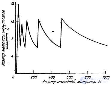
Fig. 11.3.2. Comparison of the effectiveness of two methods of obtaining the final convolution: direct and with the Fourier transform.

The calculation of the convolution with the Fourier transform requires a smaller number of operations than in the case of its direct calculation, if the length of the impulse response is large enough. However, if the processed image is also large, the relative efficiency of the method using the Fourier transform decreases. In addition, when calculating the Fourier transform of large matrices, difficulties arise in ensuring the accuracy of the calculations. Both problems can be resolved by resorting to block-based image filtering, when a large matrix is ​​subdivided into a series of overlapping blocks processed alternately [2, 7–9].

In fig. 11.3.3, and it is shown how the block containing the items. After convolving it with an impulse response consisting of elements, it turns out a block of size elements, which are placed in the upper left corner of the output matrix (Fig. 11.3.3, a). Next, from the processed matrix extract the next block size elements and from it receive the second block of the processed size image adjacent to the first. As shown in fig. 11.3.3, b, the second block of the original image must overlap with the first block in the strip width element. Then the processed blocks will dock without a gap. This process continues until all blocks adjacent to the top row of the matrix are processed. If the last block in this block line is incomplete, add zero elements to it. Next, remove the block located at the beginning of the second row and overlapping with the blocks of the first row in the strip width element. The process continues until all elements of the processed image have been determined.

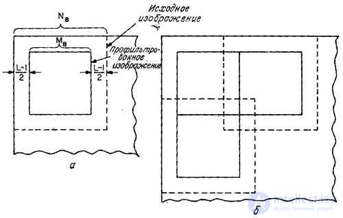
Fig. 11.3.3. Placing blocks with block image filtering.

a - the first block; b - the second blocks in the row and column of blocks.

To obtain convolution with the Fourier transform is required

(11.3.6)

operations. When block processing, when the block size is necessary

(11.3.7)

operations where the number of blocks - fraction value rounded up . Hunt [9] determined how the optimal block size depends on the size of the matrices of the original image and the impulse response.