Lecture
Introduction
Electrical engineering is a general education discipline that studies the use of electromagnetic phenomena for practical purposes, as well as issues of production, transmission over a distance, and conversion of electrical energy into other types of energy.
Basic concepts of electrical engineering
The electric field is one of the forms of manifestation of the electromagnetic field, characterized by the electric field intensity
E - emf (V)
Potential - energy of a charged particle or node
φ (B)
Voltage or potential difference
U = φа - φв (В)
Current - the directional movement of electric charges. Currents can be: constant, the value and direction of which does not change in time, variables, the value and direction of which changes in time.
I (A)
Resistance R (Ohms)
Conductivity G (Sim) 
Electrical circuit topology
a) branch - a section of an electrical circuit with the same current
branch is active 
branch passive 
The number of branches - p
b) a node - q a junction of three or more branches; nodes are potential or geometric
rice one 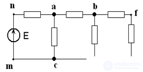
Four geometric nodes (abcd) and three potential (abc) as the potentials of nodes c and d are equal:
φс = φd
c) Contour - a closed path passing through several branches and nodes of an extensive electrical circuit - abcd, fig. 1. An independent circuit with at least one new branch.
d) Bipolar - part of an electrical circuit having two poles of the output. Bipolar networks are active and passive.
contain emf or IT 
contain only passive elements 
e) Four - port network - a part of an electrical circuit having four poles of a terminal, are active and passive.
contain emf or IT 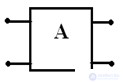
contain only passive elements 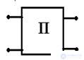
Electrical circuit and its elements
An electrical circuit is a set of generating, receiving and auxiliary devices connected by electrical wires and forming a closed path for electrical current.
Sources of electrical energy - converters of chemical, mechanical, thermal, light, etc. energies into electrical energy: 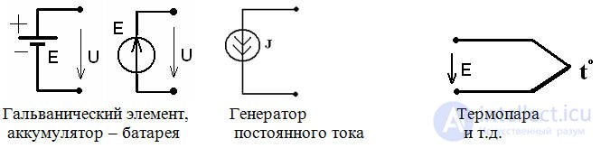
Receivers of electrical energy:
a) with irreversible processes of conversion of electrical energy into other types of energy:
Resistor, (the conductor's resistance to electric current), electrical energy is converted into heat.
Resistor symbol 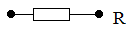
1-type device:
Р - constant, RP - variable, ТР - thermistor, etc.
2-material:
1 - non-wired, 2 - wire, etc.
3-ordinal development number
Example designation: P1-26 (fixed non-wired resistor).
The main parameters of resistors
nominal resistance and tolerance on the value of resistance
rated power
temperature coefficient of resistance
Values of nominal resistances are selected from the series of resistances Е6, Е12, Е24, Е48, Е96, Е192
Incandescent lamp, electrical energy is converted into light, heat energy, etc. 
b) with reversible processes of electrical and magnetic energy conversion
A capacitor is an element of an electrical circuit,
intended to be used by him
electrical capacitance
Symbol Capacitors 
Capacitor, with capacity
C = q / u.
Capacity of a flat capacitor 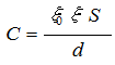
1-type device:
K- permanent, CT-trimmer, KP-variable;
2-digit, determining the type of dielectric (10-ceramic, 40-paper ...);
3-number development.
Example: K10-36 permanent capacitor ceramic
The main parameters of the capacitor
rated capacity
operating voltage
loss tangent
temperature coefficient of capacitance (TKE)
Inductor with inductance 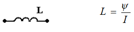
Auxiliary devices:
a) Switches that control the operation mode of the electrical circuit
b) Relay
c) fuses for protection against overvoltage or inadmissible current values.
d) Switches, switches.
Electrical Circuit Classification
Active:
Emf
Current source
Passive:
Linear: R, C, L
Nonlinear: diodes, zener diodes and d
Laws describing the operation of an electrical circuit
Ohm's law - current strength is directly proportional to the applied voltage and inversely proportional to the resistance of the conductor. 
Generalized Ohm's law for the active branch: 
Rule: EMF and voltage are taken with a “+” sign, if their directions coincide with the direction of the current, and with a “-” sign, if not.
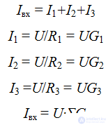
Kirchhoff's laws
1st law: the algebraic sum of the currents of the branches converging in one node is zero. Rule: the current flowing into the node is taken with a "+" and flowing with a "-".
Σ Ii = 0, for example:
I1 + I2 - I3 = 0 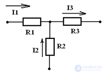
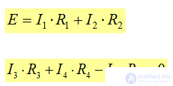
2nd law: the algebraic sum of voltages on the resistive elements of a closed active circuit macn (Fig. 1) is equal to the algebraic sum of the emf included in this circuit.
ΣRi • Ii = ΣEi
Example: Let's make an equation according to the 2nd Kirchhoff's law for 1 circuit and for 2 circuit, Fig. 1: 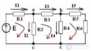
the algebraic sum of the voltages of all sections of the closed passive loop abcd (Fig. 1) is 0.
ΣUi = 0
The rule is: if the emf and current have the same direction as the circuit bypass direction, then they are taken from “+”, if not, then from “-”.
Joule-Lenz law
Power source e. energy is defined as the product of current and voltage:
Pist = U • J or Rist = E • I
The power of the receiver is defined as the product of the square of the current and the resistance of the branch:
Rpr = I² • R
Power sources of electrical circuits
Sources EMF
The equivalent circuit of a real source of EMF with a passive receiver 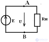
when, Rvn ≠ 0, the voltage at the terminals of the AV source is determined by the equation:
U = E – I • Rвн
The equivalent circuit of a real source of EMF with an active receiver 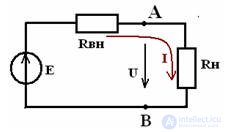
the voltage at the terminals of the AV source is determined by the equation:
U = E + I • Rвн
The replacement scheme of the ideal source of EMF 
External characteristics of the source EMF 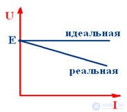
Current source
The equivalent circuit of a real current source with a passive receiver 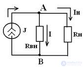
when, Rвн → ∞, the voltage at the terminals of the AV source is determined by the equation:
I = J-In; I = E • Gвн - U • Gвн
where j = e / rvn; E = J / Gvn; G = 1 / Rvn
An ideal source of current when Gvn << Gn
The load current will be equal to:
I = E • Gвн
External characteristics of the current source 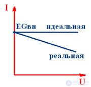
DC source operation modes
1. Idle mode corresponds to open source terminals, while the current in the load is absent I = 0, therefore Uxx = E and the power in the load
Pxx = E • I = 0
This mode is used to measure the emf source.
2. The short circuit mode is created when the source terminals are short-circuited, i.e. voltage on the load is zero, because its resistance is equal to zero Rн = 0, therefore, Un = 0 and the short-circuit current is determined: Iкз = E / Rвн = E • Gвн, usually this is an emergency mode at which Iom << Iкз, where Iom is the current for which the element is calculated . Power in the load in this case is equal to zero Рн = I² • Rн = 0.
3. Consistent operation of the source and load, when Rвн = Rн and is characterized by the maximum possible transmission power from the source to the receiver
source current
I = E / (Rvn + Rn)
source power
Pist = E • I = E² / (Rвн + Rн) = E² / 2Rвн
PH = 0.5 • Rist
receiver power (load)
Rn = UI = I² • Rn = RnE² / (Rnn + Rn) ² = E² / 4Rvn
4. Nominal mode - the operation of the source and receiver at the nominal values of the currents and voltages for which they are designed.
Power balance
We make the equations to determine the power of the receiver:
ΣRpr = Σ I² • R
Build equations for determining the power source:
ΣPist = Σ E • I
The balance converges provided that the power and receiver power equations are equal, i.e .:
ΣRpr = ΣPist
The balance is considered converged if the error of non-convergence is no more than 2%
Parallel and parallel connection
Serial connection when the current in each element is the same. 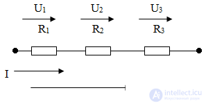

Serial connection properties:
a) The circuit current and voltage depends on the resistance of any of the elements;
b) The voltage on each of the series-connected elements is less than the input; 
c) Serial connection is a voltage divider.
Parallel connection
A connection in which all sections of a circuit are connected to one pair of nodes affected by the same voltage. 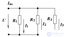
Parallel connection properties:
Equivalent resistance is always less than the smallest of the branch resistances;
The current in each branch is always less than the source current. The parallel circuit is a current divider;
Each branch is under the same source voltage.
Mixed compound
Mixed connection is a combination of serial and parallel connections.
THE METHOD OF EQUIVALENT TRANSFORMATIONS 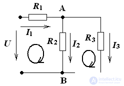
Conversion schemes always start from the end. In this example, we first apply the parallel transform. 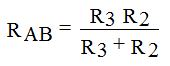
After which the scheme will look like 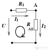
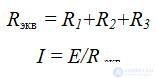
Now it remains to calculate Rack for this we apply the sequential conversion 
By calculating Rack, you can proceed to the calculations of current and voltage on a section of the circuit. 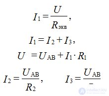
4. Connection star and triangle 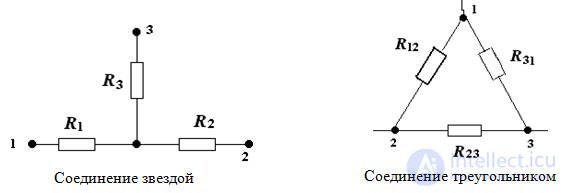
Formulas for the transition from a star to a triangle 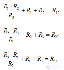
From triangle to star 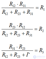
Bridge connection
The circuit is calculated by the method of an equivalent generator, if a load is connected to the output. 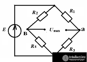
Determine Uout = φа - φв with disconnected load 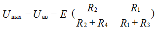
If all the resistances are the same, then the output voltage is 0
Kirchhoff method
The most accurate method, but with its help you can determine the parameters of the circuit with a small number of contours (1-3).
Algorithm:
1. Determine the number of nodes q, p branches and independent contours;
2. Set the directions of the currents and circuit rounds arbitrarily;
3. Establish the number of independent equations according to the 1st Kirchhoff's law (q - 1) and compose them, where q is the number of nodes;
4. Determine the number of equations according to the 2nd Kirchhoff's law (p - q + 1) and compose them;
5. Solving together the equations, we determine the missing parameters of the circuit;
6. According to the data obtained, calculations are verified by substituting the values into the equations according to the 1st and 2nd Kirchhoff laws, or by compiling and calculating the power balance.
Example: 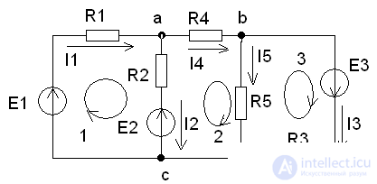
Figure 1. According to the proposed algorithm, we determine the number of nodes and branches of the circuit in Fig. one
q = 3, p = 5, therefore, the equations according to the 1st Kirchhoff’s law are 2, and the equations according to the 2nd Kirchhoff's laws are 3.
We write these equations according to the rules: 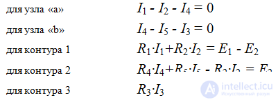
Let's make the power balance equations: 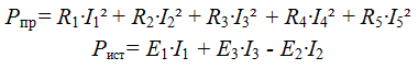
Loop current method
Using this method, the number of equations is reduced, and the equations for the first law are eliminated.
Kirchhoff's horse. The concept of a loop current is introduced (this is a virtual concept), equations are compiled according to the second Kirchhoff law.
Consider our example pic. one 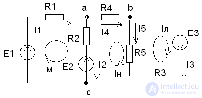
Pic.1
Contour currents are designated Im, In, Il, their directions are given, as shown in fig.
Algorithm of the decision:
1. we write the real currents through the contour: along the external branches I1 = Im, I3 = Il, I4 = In and along the adjacent branches I2 = Im - In, I5 = In - Il
2. Create equations according to the second Kirchhoff law, as there are three contours, therefore there will be three equations:
for the first circuit Im • (R1 + R2) - In • R2 = E1 - E2, the “-” sign in front of In is placed because this current is directed against Im
for the second circuit - Im · R2 + (R2 + R4 + R5) • In - Il • R5 = E2
for the third circuit - In • R5 + (R3 + R5) • Il = E3
3. Solving the resulting system of equations, we find the contour currents
4. Knowing the contour currents, we determine the actual currents of the circuit (see paragraph 1.
Nodal potentials method
The proposed method is the most effective of the proposed methods, while the accuracy of the calculations is of course lost, this method is incorporated into the engineering programs of the EWB MULTISIM, TINA, definitions of the circuit parameters.
The current in any branch of the circuit can be found by the generalized Ohm's law. For this it is necessary to determine the potentials of the nodes of the circuit.
If the scheme contains n-nodes, then the equations will be (n-1):
Ground any node of the circuit φ = 0;
It is necessary to determine the (n-1) potentials;
Equations are compiled according to the first Kirchhoff law according to the type: 
where I11 ... I (n-1), (n-1) the node currents in the branches with EMF connected to this node, Gkk is the sum of the conductances of the branches in node k, called the intrinsic conductivity, Gkm is the sum of the conductances of the branches connecting the nodes k and m, taken with a “-” sign, called mutual conductivity between nodes;
The currents in the circuit are determined by the generalized Ohm's law.
Example: 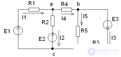
Ground the node C, i.e. φс = 0 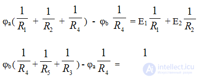
Defining the potentials of φа and φb, we find the currents of the circuit. The compilation of formulas for calculating currents is carried out in accordance with the rules of EMF signs and voltages, when calculating according to the generalized Ohm law. 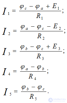
The correctness of the calculation of currents is checked using the laws of Kirchhoff and the power balance
Two node method
The method of two nodes is a special case of the method of nodal potentials. It is used when the circuit contains only two nodes (parallel connection).
Algorithm:
Positive current directions and voltages between two nodes are arbitrary;
Equation for determining inter-nodal voltage 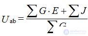
where G - branch conductivity, J - current sources;
Rule: G • E and J are taken with a “+” sign if E and J are directed to a node with high potential;
The currents of the circuit are determined by the generalized Ohm's law.
Example: 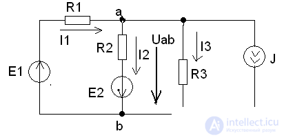

The compilation of formulas for the calculation of currents is carried out in accordance with the rules of EMF signs and voltages, when calculating according to the generalized Ohm's law. 
Active two-pole method (generator)
This method is used when it is necessary to calculate the parameters of one branch in a complex scheme. The method is based on the active two-terminal theorem: “Any active two-terminal network can be replaced by an equivalent two-terminal network with parameters Еэкв and Рэкв or Jэвв and Geqв, the mode of the circuit will not change.”
Algorithm:
Open the branch in which you want to define parameters.
Determine the voltage at the open terminals of the branch, i.e. with idle mode Eekv = Uxx favorite method.
Replace active bipolar, i.e. the circuit without the branch under study is passive (exclude all power sources, leaving their internal resistances, not forgetting that the ideal EMF has Rvn = 0, and that of the ideal current source Rvn = ∞). Determine the equivalent resistance of the resulting circuit RACK.
Find the current in the branch by the formula I = Eeqv ((R + Rekv) for the passive branch and I = E ± Eeqv / (R + Reqv) for the active branch
Nonlinear dc circuits
Definition of nonlinear element
In practice, in industrial electronics, electrical circuits consist mainly of nonlinear elements, i.e. of elements whose current-voltage characteristics are not a straight line (the parameter values change drastically with current)
All non-linear CVCs have all semiconductor devices:
Semiconductor diodes, zener diodes, thermistors, transistors, thyristors, etc.
The analysis and calculation of nonlinear circuits is carried out using the method of intersection of characteristics, the equivalent method, of an active two-port network.
Characteristics and parameters of the nonlinear element
The concepts of static and dynamic (differential) resistance 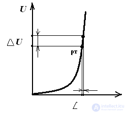
Pic 1
Rct = Urt / Ipt - the ratio of the voltage on the element to the current at a given point of its characteristics
Rdin = dU / dI = ∆U / ∆I - the ratio of the change in voltage to the change in current in a given working area of a nonlinear element Rst> Rdin
Nonlinear Circuit Analysis
It is carried out in two ways analytically or graphically - by intersecting the characteristics - this is the solution of the non-linear equation determining the electrical state in a graphical way.
Consider a chain section with series-connected linear and non-linear elements.
(pic 2). 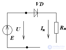
Pic 2 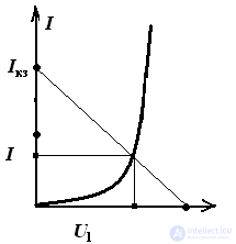
Pic 3
We make the equation of the electric state for the circuit of Fig.2:
U = E - Rn • I
According to this equation, the “inverted” I – V characteristic of the resistor RH (or the load line) is constructed.
Rule: if a nonlinear element is connected in series with a resistor, then an “inverted” I – V characteristic is constructed; if in parallel, then a normal I – V characteristic of the resistor is constructed.
As you know, any straight line is built on two points, which correspond to two modes of a two-terminal network with parameters E and Rn.
Idling: I = 0; U = E
Short circuit: U = 0; Ikz = E / Rn
The intersection of the current-voltage characteristics of the nonlinear element and the resistor give a graphical solution to the problem, as shown in Fig. 3
In the analysis of nonlinear circuits, an equivalent generator method is used, in the case of a complex circuit: A multi-element active linear two-pole network, to the output terminals of which a non-linear element is connected, can be replaced by an equivalent two-pole network. The voltage and current on the nonlinear element are found by intersecting characteristics, knowing these parameters you can determine the currents and voltages of the other branches of the circuit.
In the case of series-connected nonlinear elements, firstly, the IV characteristics of the elements are graphically folded, and then the calculation is carried out as shown earlier.
The addition of the current-voltage characteristics, with the sequential inclusion of nonlinear elements 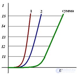
Addition of VAC, with parallel connection of nonlinear elements 
Sine of sinusoidal current
Modern electric power industry is based mainly on alternating current. The introduction of alternating current into practice dates back to the 70s of the 19th century.
По сравнению с другими токами синусоидальный имеет ряд преимуществ, которые позволяют экономично осуществляет производство, передачу, распределение и использование электрической энергии. В настоящее время производство и передача электрической энергии осуществляются при помощи трехфазного тока с частотой 50 Гц во всех странах мира кроме США и Японии (60Гц).
Различные области техники используют широкий диапазон частот синусоидального тока, в зависимости от технических потребностей. Так в авиации применяют синусоидальный ток с частотой 400 Гц, так как при этом снижаются габаритные размеры и вес оборудования. В электротермических установках используют диапазон частот от 500Гц до 50МГц. Частоты от долей Гц до 10ГГц применяют в радиотехнике.
Но с использованием синусоидального тока появляются электромагнитные процессы, оказывающие влияние на электрические цепи более сложного характера, чем в цепях постоянного тока. Появляется ряд особенностей в работе, например, конденсатора и катушки индуктивности. Переменный ток порождает в этих элементах переменные электрическое и магнитное поля. В результате возникают явление самоиндукции в дросселе и токи смещения в конденсаторе, которые оказывают существенное влияние на процессы в сложных электрических цепях.
Параметры синусоидальных электрических величин
Синусоидальная функция является периодической функцией времени, т.е. через равный промежуток времени, называемый периодом T, цикл коле***ний повторяется.
i(t) = i(t + T), где i - мгновенное значение тока
Периоду Т соответствует фазовый угол 2π или 360°. Длительность времени периода Т измеряется в секундах.
Величина обратная периоду Т называют частотой и измеряется в Гц (число периодов в секунду) 
Также используется угловая частота ω =2πƒ (рад/сек) показывающая насколько фазовый угол синусоиды изменился за период, т.е. скорость изменения фазового угла синусоиды.
Аналитическое выражение мгновенных значений тока, ЭДС и напряжения определяется тригонометрической функцией:
i(t) = Im sin(ωt + ψi)
u(t) = Um sin(ω t + ψu)
e(t) = Em sin(ωt + ψe),
где Im, Um, Em – амплитудные значения тока, напряжения и ЭДС;
(ωt + ψ) – аргумент синуса, который определяют фазовый угол синусоидальной функции в данный момент времени t;Ψ – начальная фаза синусоиды, при t = 0
По ГОСТу ƒ = 50 Гц, следовательно, ω = 2πƒ = 314 рад/сек.
Временную функцию можно представить в виде временной диаграммы, которая полностью описывает гармоническую функцию, т.е. дает представление о начальной фазе, амплитуде и периоде (частоте). Временные диаграммы можно наблюдать с помощью специального прибора – осциллографа.
Рассмотрим пример: 
Функция тока i(t) сдвинута вправо от начала координат, это означает, что начальная фаза имеет отрицательный угол, ток появляется раньше на ψi относительно начала координат. Ток опережает начало координат
Но аналитическое выражение запишется следующим образом:
i(t) = Im sin(ωt + ψi),
Знак «+» или «–» перед начальной фазой показывает, сколько не хватает градусов, чтобы наша функция выходила из начала координат. Начальную фазу отсчитывают от начала синусоиды, при t = 0, до начала координат.
Все сказанное выше относится и к функциям напряжения u(t) и ЭДС e(t)
При рассмотрении нескольких функций электрических величин одной частоты интересуются фазовыми соотношениями, называемой углом сдвига фаз.
Угол сдвига фаз φ двух функций определяют как разность их начальных фаз φ = ψu - ψi
Если начальные фазы одинаковые, то φ = 0, тогда функции совпадают по фазе;
Если φ = ± π, то функции противоположны по фазе.
Особый интерес представляет угол сдвига фаз между напряжением и током рис.5 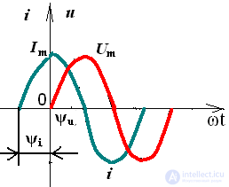
Pic.5
На практике используют не мгновенные значения электрических величин, а действующие значения. Действующим значением называют среднеквадратичное значение переменной электрической величины за период. Обозначается той же буквой, что и амплитудное значение, но без индекса. 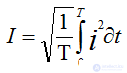
Для синусоидальных величин действующие значения меньше амплитудных в  раз, т.е.
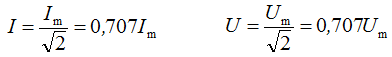
Электроизмерительные приборы градуируются в действующих значениях.
Часто для технических расчетов необходимо знать среднее значение электрических величин, но его берут за половину периода, так как при определении среднего значения за период у синусоидальной функции получается 0. 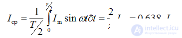
Следует обратить внимание на то, что среднее значение меньше действующего
Применение комплексных чисел для расчета электрических цепей
Расчет электрических цепей с использованием тригонометрических функций весьма сложен и громоздок, поэтому при расчете электрических цепей синусоидального тока используют математический аппарат комплексных чисел. 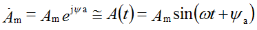
Модуль комплексной амплитуды равен амплитуде синусоидальной величины, а аргумент – ее начальной фазе.
Вводится понятие комплексного величин амплитуд и действующих значений тока, напряжения, ЭДС и т.д. 
Комплексные действующие значения пропорциональны комплексным амплитудам и записываются в виде: 
Синусоидальные электрические величины, представленные в комплексной форме, можно изображать графически. На комплексной плоскости в системе координат с осями +1 и +j, которыми обозначены положительные действительная и мнимая полуоси, строятся комплексные векторы. Длина вектора пропорциональна модулю действующих значений. Угловое положение вектора определяется аргументом комплексного числа. При этом отсчет положительного угла ведется против часовой стрелки от положительной действительной полуоси. Комплексная плоскость разбивается на четыре четверти: 
Итак, рассмотрим нашу тригонометрическую функцию A(t) представленную в виде комплексной величины на комплексной плоскости. Получается, что наша функция представлена в виде вектора вращающегося на комплексной плоскости против часовой стрелки со скоростью ω, как показано на рис.1. 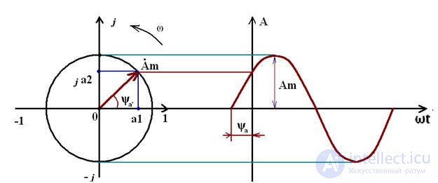
Pic.1
Из рис.1 видно, что вектор на комплексной плоскости можно построить двумя способами, первый, зная размер вектора и угол, и второй способ, зная координаты вектора по действительной и мнимой осям.
Первый способ это показательная форма представления комплексного числа, т.е. 
где - комплексная величина, А - модуль комплексного числа или действующее значение величины, ψа - аргумент комплексного числа
Второй способ алгебраическая форма представления комплексного числа: 
где а1 = Асоs ψа а2 = Аsin ψа
Правила перехода из одной формы в другую.
Переход из показательной формы в алгебраическую форму:
дано 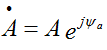
Используется формула Эйлера 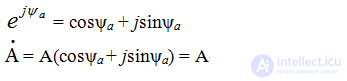
Переход из алгебраической формы в показательную форму:
дано 
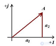
Fig. 2
Из рис.2 видно, вектор образует с осью координат прямоугольный треугольник, поэтому воспользуемся теоремой Пифагора, и найдем размер вектора, который равен гипотенузе треугольника: 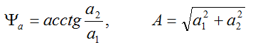
причем особое внимание уделим углу – аргументу ψа модуля комплексного числа:
если вектор находится во второй и третьей четвертях комплексной плоскости, то к полученному значению аргумента необходимо прибавить 180° или π.
Если а1 = 0, то комплексное число называется мнимым, аргумент ψа = ± 90°
Если а2 = 0, то комплексное число называется действительным, ψа = 0, ± π
Простейшие математические операции с комплексными числами
Простейшие математические операции такие, как сложение, вычитание, умножение и деление проводятся с комплексными числами следующим образом: сложение и вычитание удобно проводить в алгебраической форме, а умножение и деление в показательной.
Единичные комплексы 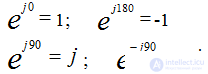
действия с j 
Векторные диаграммы синусоидальных функций
Геометрический образ комплексных величин синусоидальных функций на комплексной плоскости называют векторной диаграммой. Векторные диаграммы широко используют для анализа электрических цепей.
Рассмотрим пример:
Given: 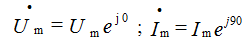
Построим векторную диаграмму на комплексной плоскости: 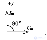
Анализируя векторную диаграмму можно сделать вывод, что функция тока опережает функцию напряжения на угол 90°.
Точно так же будет выглядеть векторная диаграмма действующих значений
Только размеры векторов уменьшаться в раз.
Рассмотрим второй пример:
На рис.3 показан узел электрической цепи и приведена векторная диаграмма токов. Необходимо определить ток I0 и построить векторную диаграмму токов. 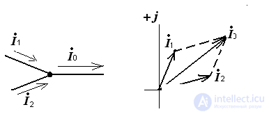
Pic.3
Ток 0 по известным токам 1 и 2 на векторной диаграмме определяется в соответствии с первым законом Кирхгофа по правилу параллелограмма.
Сопоставление диаграмм доказывает важность фазовых соотношений в цепях переменного тока, потому что, при неизмененных амплитудах (действующих значениях) суммируемых токов или напряжений результирующие величины этих токов и напряжений существенно отличаются по амплитудам за счет различия в фазовых соотношениях
Комплексное сопротивление
Введем понятие комплексного сопротивления, которое определяется отношением комплексной амплитуды напряжения к комплексной амплитуде тока. 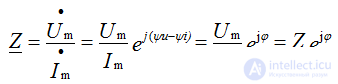
Модуль комплексного сопротивления, равен отношению амплитуды напряжения к амплитуде тока: 
Комплексное сопротивление выражается через комплексные действующие значения напряжения и тока: 
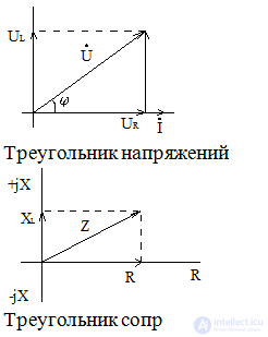
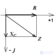
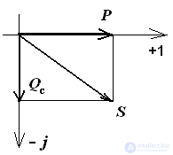
Треугольник сопротивлений 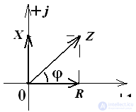
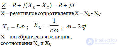
В алгебраической форме Z = R + jX,
Where:
R - активное сопротивление,
X - реактивное сопротивление,
R = Zcosφ, R≥0,
X = Zsinφ, причем реактивное сопротивление может быть как положительным так и отрицательным или равное нулю. Таким образом, вектор полного комплексного сопротивления может находиться только в 1 или 4 четвертях комплексной плоскости
Мощности в цепях переменного тока
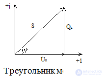
Полная комплексная мощность 
 - комплексное действующее значение напряжения
  - сопряженный комплекс тока
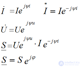
где модуль полной мощности S = U•I
размерность полной мощности - (BA)
В алгебраической форме полная мощность имеет вид:
S = UIcosφ + jUIsinφ,
P = UIcosφ - активная мощность Вт
Q = UIsinφ - реактивная мощность ВАр
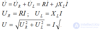
Chains with R, C, L elements
Electrical circuit with R-element 
Pic.1
Consider a circuit with an R-element, as shown in Figure 1. Place the directions of current and voltage and write down the electric equations of this circuit according to Ohm’s law:
i = u / R = (Um / R) sin (ωt + ψu) = Imsin (ωt + ψi)
it is obvious that Um = RIm; ψu = ψi, then the phase angle between voltage and current will be 0, i.e.
φ = ψu - ψi = 0, which corresponds to the time diagram shown in Figure 1, the voltage and current coincide in phase.
For valid values Ohm's law: U = RI 

the impedance of the resistive element is always a valid positive number, which is equal to the active resistance value R.
Power on R-element:  phase angle φ = 0, then P = UIcosφ = UI, Q = UIsinφ = 0, therefore, the total power on the resistive element is equal to the active power. This means that the resistor is working to convert electrical energy into heat.
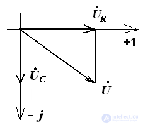
Electrical circuit with capacitive C - element
An ideal capacitor when its active resistance is Rc = 0. 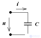
u (t) = Um sin (ωt + ψu)
i = = C = C • ω • Umcos (ωt + ψu)
i = C • ω • Umsin (ωt + ψu + 90 °)
initial current phase ψi = ψu + 90 °
From the vector diagram shows that the current on the capacitor is ahead of the voltage by 90 ° 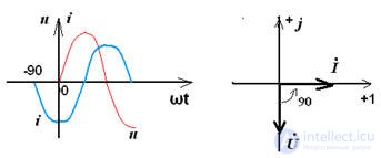
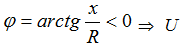
 , since φ = -90 °,
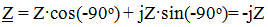
and the module impedance 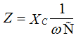 ,
,
therefore, the capacitor resistance is purely reactive and is: 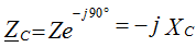 .
.
Ohm's Law: U = I • (-Xc)
Power on C - element:  phase angle φ = -90 °,
then P = UIcosφ = 0, Q = UIsinφ = -UI, therefore on the C - element energy is exchanged between the source of electrical energy and the electric field of the capacitor, which determines the reactive power Q.
C - the element of work does not make, therefore the active power is equal to 0. 
Electrical circuit with inductive L - element
The ideal inductor has an active resistance of RL = 0.
i (t) = Imsin (ωt + ψi)
eL = - L = - LωImcos (ωt + ψi)
eL = Emsin (ωt + i + 90 °)
u = - eL;
u (t) = Um sin (ωt + ψu) 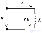
initial phase ψu = ψi + 90 °
phase angle φ = ψu - ψi = 90 ° 
It can be seen from the vector diagram that the voltage on the inductance voltage is ahead of the current by 90 °, since φ = 90 °, then 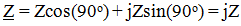 ,
,
and the modulus of complex resistance is Z = XL = ωL, therefore, the resistance is purely reactive and is: 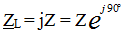
Ohm's Law: U = I • (XL)
Power on L - element:  the phase angle φ = 90 °, then
P = UIcosφ = 0, Q = UIsinφ = UI, therefore on the L - element there is an exchange of energy between the source of electrical energy and the magnetic field of the coil, which determines the reactive power Q. L - element does not perform work, therefore the active power is 0. 
A real coil has an active resistance determined by the resistance of the wires, therefore the total impedance is equal to: 
Analysis of sinusoidal current circuits
1. Analysis of sinusoidal current circuits occurs under the condition that all elements of the circuit are ideal, i.e. R, L, C are perfect.
The electrical state of sinusoidal current circuits is described by the same laws as in DC circuits.
Ohm's law: 
Kirchhoff's first law in trigonometric form: 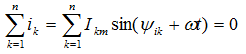
Kirchhoff's first law in a complex form: 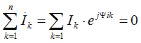
Kirchhoff's second law in trigonometric form: 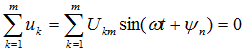
Kirchhoff's second law in a complex form: 
The algebraic sum of the complex voltages on the passive elements is equal to the sum of the external emfs included in this circuit. m is the number of contour plots. The rules of signs when drawing up equations are the same as in DC circuits.
Sequential connection of elements in a sinusoidal current circuit:
RLC circuit 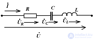
According to the second law Kirchhoff in an integrated form 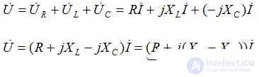
Ohm's law 

Zekv - module of equivalent resistance (impedance determines the connection between U and I)  - argument, connection between initial phases
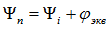
Triangles of resistance and voltage 
From the triangle: 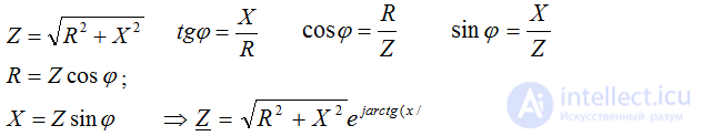
Stress triangle 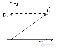
Chain rl 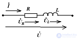
RL circuit power 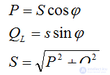
RC circuit 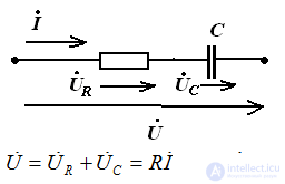
Resistance Triangle Voltage Triangle Power Triangle 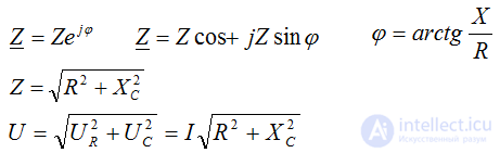
If the circuit consists of series-connected elements with active and reactive resistance, then the vector diagram has the form of a right triangle.
Voltage resonance
The mode of operation of the RLC circuit or LC circuit, provided that the reactances XC = XL are equal, when the total voltage of the circuit coincides in phase with its current, is called voltage resonance.
XC = XL - resonance condition 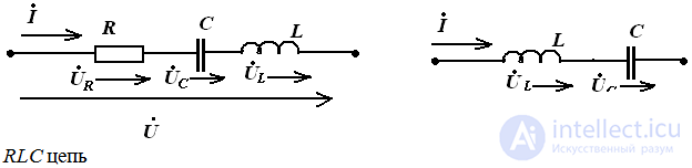
Signs of voltage resonance:
The input voltage is in phase with the current, i.e. phase shift between I and U φ = 0, cos φ = 1
The current in the circuit will be greatest and, as a result, Pmax = I2maxR is also maximum, and the reactive power is zero.
Resonance frequency 

Resonance can be achieved by changing L, C or ω.
Vector diagrams at voltage resonance 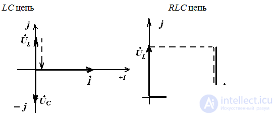
Cases of other modes of operation of the RLC circuit
If XL> XC ie 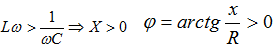
U is ahead of I, so the circuit is actively inductive.  the voltage on the coil is greater than the voltage on the capacitor.
Vector diagram 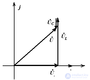
If XL <XC, i.e. 
 lags behind I, then the circuit has an active-capacitive character
the voltage on the capacitor is greater than the voltage on the coil.
Vector diagram 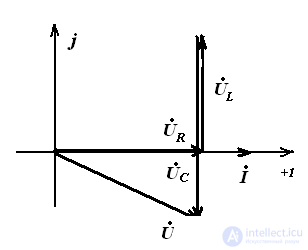
Parallel connection of elements in a sinusoidal current circuit 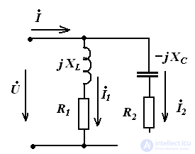
At the input of a parallel circuit voltage U
Ohm's law 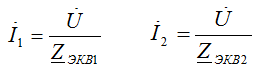
Equivalent branch resistances: 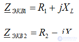
We write the equivalent conductivity: 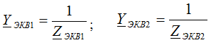
according to the first Kirchhoff law: 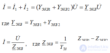
Triangles of conductivity and currents
algebraic form 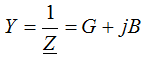
G - the real part, the active component
B - imaginary part, reactive component. 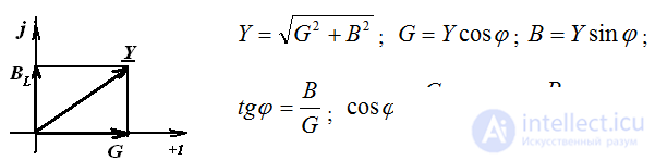
Conduction triangle 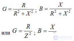
Current triangle 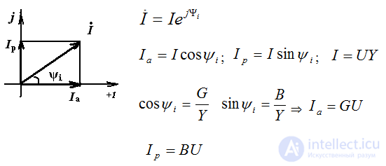
Current resonance
The mode in which the circuit containing parallel branches with inductive and capacitive elements, the current unbranched part of the circuit coincides in phase with the voltage (φ = 0), is called the resonance currents.
Current resonance condition: 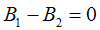
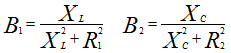
B1 - reactive conductivity of the first branch,
B2 - reactive conductivity of the second branch
Signs of current resonance:
The reactive components of the branch currents are IPC = IPL and are out of phase in the case when the input voltage is purely active;
The currents of the branches exceed the total current of the circuit, which has a minimum value;
and match in phase 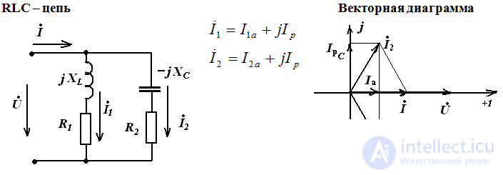
Resonance frequency 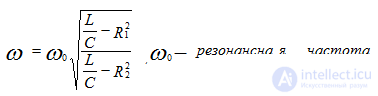
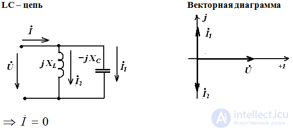
Cases of resonant circuits 
If R2 = 0 resonance occurs when 
Current Resonance Cases
Case 1. One resonance in the circuit, provided: 
Case 2. Two resonances in the circuit, at a certain ratio of the resistances of the elements. 
Case 3. No resonance in the circuit - the frequency is an indefinite value, with 
Frequency characteristics of the null *** body contour 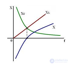

Power balance in AC circuits 
Power factor
It is energetically advantageous to operate a generator or electrical equipment if it performs the maximum work. Work in the electric circuit is determined by the active power R.
Power factor indicates how efficiently a generator or electrical equipment is used.
λ = P / S = cosφ≤1
With a decrease in the power factor, the cost of consumption of *** electric power increases.
Ways to increase power factor
Power is maximum in the case when P = S, i.e. in the case of a resistive circuit.
The generator performs only irreversible energy transformations and does not participate in collective energy exchange processes with the electromagnetic field of the receivers, in the maximum power mode.
Consumers of electrical energy basically have an RL element replacement circuit, therefore, an increase in power factor is possible by compensating reactive power by connecting a capacitive element (QL-QC), connecting a capacitive element reduces the current in the transmission line, which reduces the cross section of the electrical wires, and this leads to savings conductive materials.
The value of the power factor in power systems depends on how competently operated electrical installations and devices.
cosφ may decrease if the units are idling or underloaded
Steady-state modes in non-sinusoidal current circuits
Representation of periodic non-sinusoidal signals
In addition to sinusoidal currents and voltages, non-sinusoidal periodic currents and voltages are widely used in electronics.
For example, rectifiers have single and full-wave instantaneous values of currents and voltages. 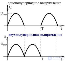
Or GLIN (generators of linearly varying voltages) and the multivibrator output have a sawtooth voltage or U - a rectangular shape. 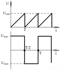
Periodic non-sinusoidal functions of time f (t) for any t must satisfy the condition: 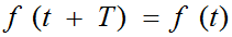 , where T is the period of coli *** days.
A vivid way to represent non-sinusoidal values are curves and their instantaneous values, which can be seen on an oscilloscope.
The second way is to represent these functions in the Fourier trigonometric series. 
The Fourier trigonometric series converges quickly, so for engineering calculations the number of harmonics is limited to 3-5 members of the series.
For example, the voltage across a half-wave rectifier load resistor. 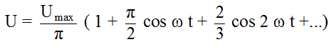
Sawtooth voltage: 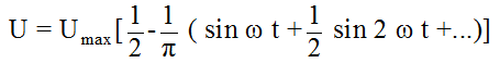
Rectangular voltage: 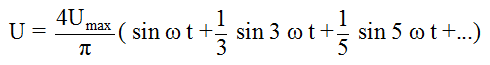
Harmonic is when a non-sinusoidal function can be decomposed into the simplest sinusoidal functions, differing in amplitude, frequency and phase
Effective and average non-sinusoidal values
Non-sinusoidal function is characterized by the following parameters:
im maximum value
effective value I
average modulo value Iср
and the constant component of Io
The effective value of a non-sinusoidal electrical quantity (determined by its root-mean-square value over a period) is equal to the square root of the sum of the squares of the constant component and the actual values of all harmonics.
Valid: 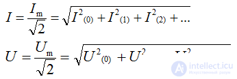
Average by module: 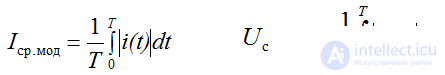
Permanent component: 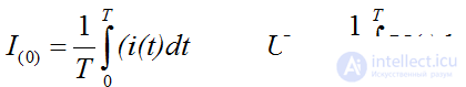
The coefficients characterizing the non-sinusoidal signals
Amplitude factors  for sinusoidal
  the sharper the curve, the larger the ka.
Form factors 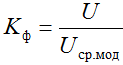 for sinusoidal values
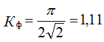
The coefficient of distortion KI = U1 / U
Harmonic factor KG = Ug / U
harmonics actual value 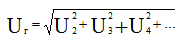
Non-sinusoidal coefficient Kp
Pulsation coefficient p is determined by the ratio of the amplitude of the first (main) harmonic to the constant component 
This coefficient is used to estimate the content of the variable component in the voltage and current curves of the rectifiers.
Transients in electrical circuits
The concept of transients. Conditions for the occurrence of transients .
Electromagnetic processes that occur in an electrical circuit, when moving from one steady state to another, are called transient.
Transients are caused by changing circuit parameters, most often as a result of commutation in a circuit. Switching (switching) is the process of closing and opening switches.
Physically, the occurrence of transients is explained by the fact that a change in the energy of electromagnetic fields cannot occur instantaneously (abruptly) in such elements as a capacitor and an inductor, since These are inertial elements.
Transition time is much less than hundredths of a second.
Equations for solving transients.
i per = iust + isc
Upper = Uust + Uсв
iy and Uy are found for a steady process, i.e. when the transition is complete.
ICB and ICB - are located when there is no energy source in the circuit, i.e. i and U are determined only by the parameters of the circuit elements.
The equations are solved on the basis of two switching laws.
The first law of commutation
The current in the branch with the inductive coil cannot change abruptly. At the first moment, the transient current retains the value that it had at the moment preceding the switching, i.e. i (0-) = i (0+). 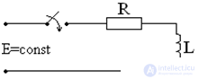
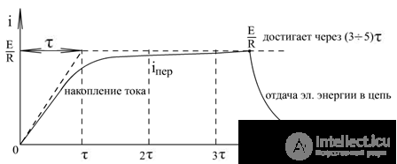
I = 0 ÷ E / R
in t (0-) → I = 0
in t (∞) → I = E / R
This conclusion was made on the basis of the impossibility of an instantaneous change in electrical and magnetic energy.
Those. let the current in the inductance change abruptly, then: 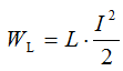
and the stored energy must also change abruptly.
Because 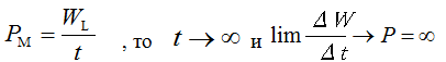
But the power can not be infinitely large, so the current in the coil can not change abruptly in contrast to the voltage. 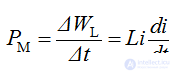
Second law of commutation
The voltage across the capacitor cannot change abruptly, i.e. U (0-) = U (0+)
Consider the RC circuit 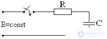
The equation according to the second Kirchhoff law:
E = iR + Uc
t (0-) → Uc (0-) = 0
t → ∞ Uc = E
Evidence:
Suppose that Uc changed abruptly, then 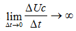 therefore, an infinitely large electrical power cannot be.
Transients in RL - chain
key closure 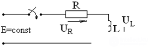
In accordance with the first law of commutation: 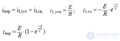
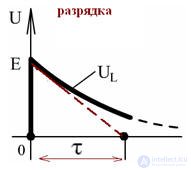
Unlike the current, the voltage on the coil changes abruptly.
- the time of accumulation of energy in the magnetic field of the coil, that is, when ↓ R and ↑ L increases τ. 
after opening 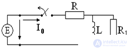
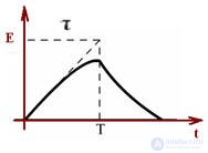
Transient use
Voltage pulse generator 

E = 10 B
E = 10 B
R = 10 ohm
R1 = 10 kΩ
Since R1 >> R
Before opening: 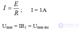
Umax = IR1 = Umax pulse = 10 kV
Used in airplanes
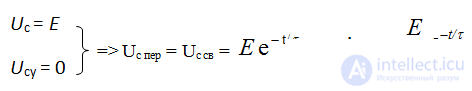
RC transient processes
The key is closed.
2nd law of commutation. 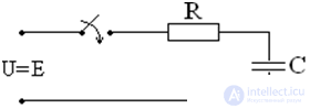
Uc = Us mouth + Uc cv
Uc mouth = E 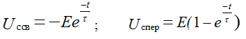
τ = RC - characterizes the speed of the transition process. The transition process will end in about (3 ÷ 5) τ. Unlike the voltage, the current on the capacitor changes abruptly. 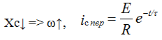
The key is open 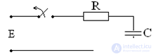
the current in the RC circuit is limited only by the resistance.
Application of the transition process in the RC circuit
Current pulse generator 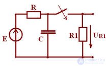
R1 << R
because R1 is small, then I ↑, EMF is not large. Capacitor C charged to EMF E. 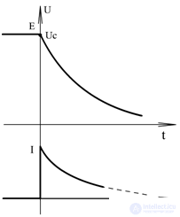
Before the key is closed, the capacitor charges to Uc = E, since R >> R1
After closing the key at the first moment R1 a little current is very large. The surge current I is called a pulse.
It is used, for example, when translating the arrows of trams and electric trains. 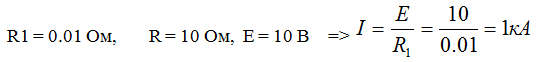
Transient processes in AC circuits.
Consider a different case.
1. τ = T
When the EMF is, the capacitor is charged, when the EMF is not - the discharge of the capacitor through R,
τ = RC 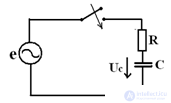
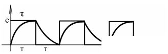
2. τ << T 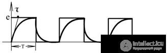
3. τ >> T 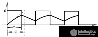
Steady-state modes in three-phase circuits
General characteristics of three-phase circuits.
It is a set of three electrical circuits in which sinusoidal electromotive forces of the same frequency act, differing in phase and created by a common energy source.
Three-phase circuits have several advantages compared with single-phase circuits:
1. Cost Effective Transmission
2. The possibility of obtaining a circular torque of the magnetic field
3. Two voltages in one installation
A three-phase circuit consists of three main elements:
1. Three phase generator
2. Transmission lines
3. Receivers 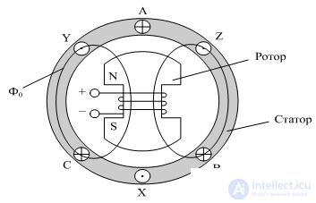
Pic 1
The windings of the generator AX, BY and CZ.
At power plants, a three-phase EMF system is formed at the terminals of a three-phase synchronous generator.
Генератор состоит из (рис. 1):
1. Неподвижный статор с тремя обмотками.
2. Вращающийся ротор (электромагнит)
Между статором и ротором находится воздушный зазор, от чего магнитный поток Фо распределяется по синусоидальному закону по окружности рис 1.
Ротор электромагнит, возбуждаемый постоянным током, вращается под действием приводного двигателя. 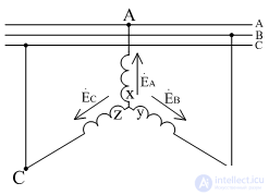
На статоре расположена обмотка, состоящая из трёх катушек или фаз, каждая из которых изображается витком. Оси катушек сдвинуты относительно друг друга на один и тот же угол 2π/3 относительно друг друга, т.е. на 120°.
Начала фаз обозначают ABC, концы XYZ.
При вращении ротора турбиной, создаваемое им магнитное поле возбуждает в неподвижных обмотках статора синусоидальные ЭДС, с одинаковой амплитудой и частотой, но сдвинутые на угол 120° (2π/3).
Эта система является симметричной.
Изображение 3х- фазного генератора рис 2 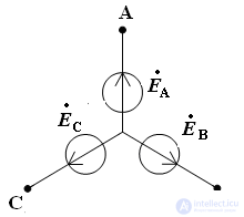
Рис 2
Тригонометрическая запись фазных ЭДС: 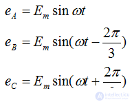
Комплексные действующие значение ЭДС: 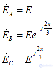
В распределительных устройствах шины различных фаз имеют различную окраску
жёлтый – фаза A
зелёный – фаза B
красный – фаза C 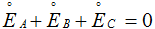 because система симметрична
Векторная диаграмма симметричного трёхфазного генератора 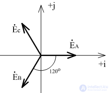
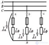
Соединение обмоток источника и фаз приёмника звездой с нейтральным проводом
(четырехпроводная сеть) 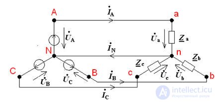
Точки n и N соединены, следовательно потенциал точки n равен 0. 
Фазные напряжения приёмника равны фазным напряжением генератора, т.е. 
соответственно, равны и линейные напряжения. Таким образом, к приёмнику, соединенному звездой подводятся два напряжения: фазное и линейное, а фазный ток равен линейному по свойству последовательного соединения  .
.
Симметричная и несимметричная нагрузка
При симметричной нагрузке когда 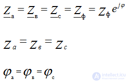
Несимметричная нагрузка 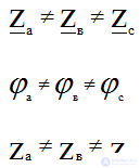
Токи при несимметричной и симметричной нагрузке
Режим каждой фазы не зависит от режима двух других фаз – ток определяется параметрами приёмника этой фазы, т.е. 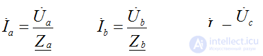
Ток в нейтральном проводе равен сумме токов фаз по 1-ому закону Кирхгофа: 
Применяется четырехпроводное включение при несимметричной нагрузке т.к., при изменении работы одной фазы режимы других фаз не изменятся, т.к. нейтральный провод обеспечивает постоянство фазных напряжений.
Токи в фазах имеют одинаковые значения по модулю и сдвинуты по фазе относительно соответствующих фазных напряжений на один и тот же угол φ, т.е. образуют на комплексной плоскости симметричную трёхфазную систему векторов.
Токи при симметричной нагрузке.
По 1-ому закону Кирхгофа при симметричной нагрузке: 
остроение векторных диаграмм
φn= φN = 0 совпадают с началом координат. Вектор фазных напряжений удобно направлять противоположно условно-положительно направлению напряжений. 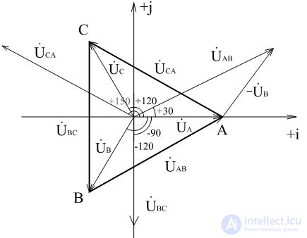
Для нахождения  необходимо к
  с противоположным знаком прибавить
  .
.
Соединим А с В, получим вектор  etc. for
  and
and  .
.
Векторы фазных напряжений образуют звезду.
Векторы линейных напряжений образуют равносторонний треугольник.
Сумма линейных напряжений всегда равна 0 
Треугольник равносторонний, следовательно , т.е. 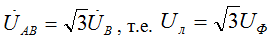
Трёхпроводная цепь
Трехпроводные цепи при соединении фаз приёмника звездой без нейтрального провода называют трёхпроводной. В такую цепь можно включать только симметричные приёмники (трёхфазные электродвигатели, электрические печи). 
Если приёмник несимметричен, то появляется напряжение смещения между нейтральными точками генератора и приемника 
Это напряжения можно определить методом двух узлов 
Напряжения на фазах приёмника неравны напряжениям на фазах генератора 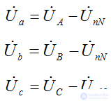
Those. при изменении сопротивления в одной фазе будут изменяться все фазные токи и напряжения, т.е. фазные напряжения приёмника не равны фазным напряжениям источника из-за смещения нейтрали, следовательно, токи тоже не будут равны.
Несимметричной нагрузкой является, например, трёхфазные трёхэлектродные дуговые печи.
Напряжения на фазах приёмника не равны напряжениям на фазах генератора.
При изменении сопротивления в одной фазе будут изменяться все фазные токи и напряжения, т.е. фазные U приёмника не равны фазным напряжениям источника из-за смещения нейтрали. 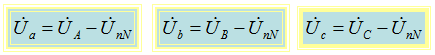
В случае симметричного приёмника достаточно определить ток в одной фазе
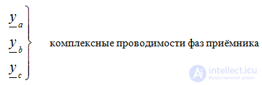
Соединение фаз приемника треугольником
Один из основных способов заметного изменения мощности при отключенной нагрузке – переключение схемы соединения источника и приемника со звезды на треугольник и наоборот.
При включении начала одной фазы с концом другой с образованием замкнутого контура получают соединение треугольником. 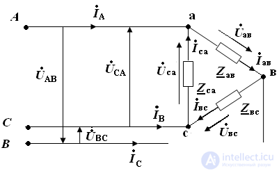
Рис 1
Соединяют треугольником фазы приемника, т.е. три фазы приемника включены между линейными проводами рис 1.
Фазные напряжения приемника равны соответствующим линейным напряжениям источника питания: 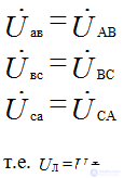
фазные токи: 
Положительное направление фазных напряжений  совпадает с положительным направлением фазных токов.
При соединении треугольником приемника получается замкнутый контур, поэтому:
Uл = Uф
Фазные напряжения определяются как линейные генератора: 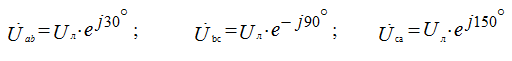
Определение фазных и линейных токов
Токи в фазах определяются по закону Ома: 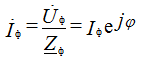
or 
Линейные токи определяются по фазным токам по первому закону Кирхгофа: 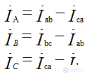
Линейные токи равны векторной разности фазных токов тех фаз, которые соединены с данным линейным проводом. 
независимо от характера нагрузки сумма линейных токов всегда равна 0.
При изменении одной из фаз режим работы других фаз остается неизменным, т.к. линейное напряжение генератора остается постоянным. Соединение треугольником используется для несимметричной нагрузки.
Векторная диаграмма токов: 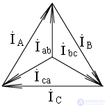
Мощности трехфазных цепей
Мгновенная мощность трехфазного источника электрической энергии:
P = P a + P b + P c = U a I a + U b I b + U c I c
Среднее за период значение мощности, т.е. мощность генератора, равна сумме активных мощностей отдельных фаз. 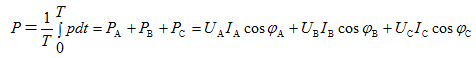
Активная мощность любой из фаз: 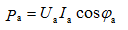
P = Pa + Pb + Pc
Реактивная мощность равна алгебраической сумме реактивных мощностей отдельных фаз:
Q = Qa + Qb + Qc
Модуль полной мощности: 
Мощность трехфазной цепи при симметричной нагрузке
Активная мощность симметричного трехфазного приемника: 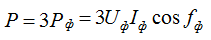
Реактивная: 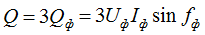
Удобнее мощности выражать через линейные Uл и Iл.
При симметричной нагрузке мощности фаз одинаковы, поэтому:
P = 3Pф = 3UфIфcosφф
Q = 3Qф = 3UфIфsinφф
S = 3Sф = 3UфIф 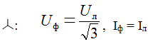
тогда 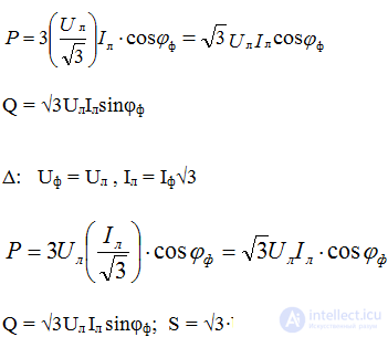
Вывод: при симметричной нагрузке формулы мощности независимо от схемы соединения приемников одинаковы
Мощность трехфазной цепи при несимметричной нагрузке
Трехфазная цепь это совокупность трех однофазных цепей, поэтому активная и реактивная мощности трехфазной цепи равны сумме отдельных фаз.
Активная мощность: 
Рассчитываются активные мощности: 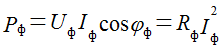
Реактивные мощности: 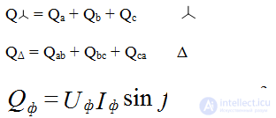
Модуль полной мощности трехфазной цепи: 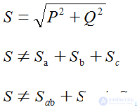 , но модули полных мощностей суммировать нельзя
Полная мощность может быть определена только в комплексной форме. 
При соединении треугольником получаем соответственно так же
Измерения в трехфазных переменных цепях
Для измерения мощности в трехфазной цепи с симметричной нагрузкой используют двух- или трех элементные ваттметры, причем:
для определения активной мощности P применяют схему включения: 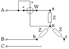
для определения реактивной мощности Q: 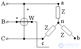
Суммарные мощности вычисляют
P = 3Pф = 3UфIф cosφ, где Pф – показание ваттметра.
В случае измерения суммарной мощности в трехфазной цепи с несимметричной нагрузкой, используют не менее двух ваттметров и результат вычисляют по формулам:
P = P1 + P2  ,
,
где P1 и P2 – показания ваттметров. 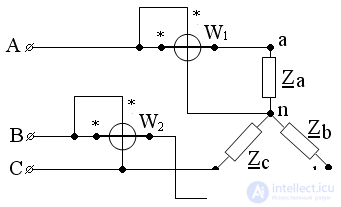
Аварийные режимы
Звезда: обрыв фазы А в трехфазной трехпроводной симметричной системе
Ya = 0 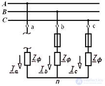
Фазные напряжения 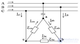
Токи в фазах приемника: 
Vector diagram 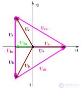
Короткое замыкание
В трехфазной симметричной системе произошло короткое замыкание фазы А приемника. При коротком замыкании фазы А сопротивление фазы 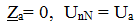
Напряжение на фазах приемника 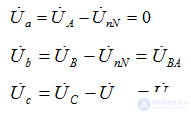
Vector diagram 
Токи в фазах В и С: 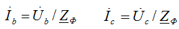
Ток фазы А находится по первому закону Кирхгофа.
Для узла n:
Обрыв линейного провода
В симметричном трёхфазном приёмнике оборвался линейный провод А
Сопротивление фазы ВС включено на полное линейное напряжение генератора, а равные сопротивления фаз 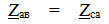 включены последовательно и к каждому из них подведена половина напряжения Uвc
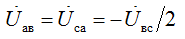
Ток фазы ВС не изменяется
Фазные и линейные токи при IA=0 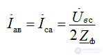
Магнитные цепи и устройства
Магнитное поле способно проявлять два действия: индукционное и электродинамическое.
Электродинамическое свойство основано на явлении электромагнитной индукции, т.е. наведение ЭДС в проводнике переменным магнитным полем. Это свойство используется в устройствах , включаемых в цепь переменного тока(дроссели, трансформаторы, электроизмерительные приборы, в устройствах постоянного тока и т.д.)
Электродинамическое действие связано с силовым воздействием магнитного поля на заряд, провод или намагниченное тело. Это действие является основным для устройств, в которых имеются подвижные элементы, и назначение этих устройств является создание механических сил (вращающих), моментов: электромагнитные реле, электродвигатели и т.д.
Усиление магнитных потоков осуществляется с помощью ферромагнетиков - рациональное использование магнитного поля.
ЭДС наводится в движущемся магнитном поле: 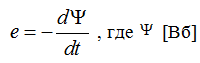 – потокосцепление катушки с магнитным полем
Направление ЭДС узнают, используя метод правой руки, когда силовые линии входят в ладонь, а отведенный большой палец указывает направление движения.
Change  может происходить в результате изменения магнитного поля или движения катушки. ЭДС настроена так, что вызванный его ток создает магнитное поле, уменьшающее изменение потокосцепления.
Basic concepts:
Магнитная индукция В (Тл) – определяет силовое воздействие магнитного поля на ток.
Намагниченность J – магнитный момент единицы объёма вещества (плотность тока).
Напряжённость магнитного поля H (А/м).
Магнитодвижущая сила (м.д.с.) F (A)
(м.д.с.) F = W•I = H∙l, м.д.с. вызывает магнитный поток в магнитной цепи. 
μо = постоянная, характеризующая магнитные свойства в вакууме. 
Магнитный поток - Ф(Вб) 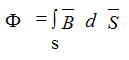
для катушки с воздушным зазором:
Ф = B•S0 = μ•H•S0
для ферромагнитных материалов, поэтому с целью уменьшения м.д.с. и уменьшения тока катушки снабжают ферромагнитным материалом (сердечником) 
Основные законы магнитных цепей
Закон Фарадея
Напряжение на катушке равно алгебраической сумме падений напряжений на сопротивлении провода обмотки и ЭДС самоиндукции 
Закон полного тока
Циркуляция напряженности магнитного поля Н вдоль любого замкнутого контура равно сумме электрических токов проводов. 
J-плотность тока
М.д.с. вдоль замкнутого контура l равна полному току Iп, пронизывающему поверхность, ограниченную данным контуром: 
Магнитная цепь – система последовательно включенных ферромагнитных и других элементов, по которым замыкается магнитный поток.
Средняя длина магнитопровода: 
Схема катушки с воздушным зазором 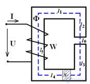
напряженность магнитного поля 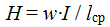
Закон Ома для магнитной цепи 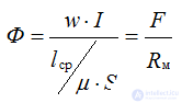
Магнитное сопротивление 
Магнитная индукция
Уравнение для источников магнитной индукции замкнутой системы 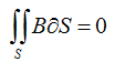
В свободном пространстве 
Для ферромагнетиков 
Технические характеристики ферромагнетиков
Для магнитных цепей с переменной м.д.с.
При подключении катушки индуктивности с воздушным зазором, к источнику переменного синусоидального напряжения, в цепи появляется переменные ток и поток.
Зависимость В(Н) - кривая намагничивания – основная характеристика ферромагнитного материала, при переменным токе перемагничивается по гистерезисной зависимости, обусловленная наличием остаточного магнетизма Br и коэрцитивной (задерживающей) силы Нс.
В однородном магнитном поле свойства ферромагнитного материала описываются гистерезисной зависимостью В(Н) 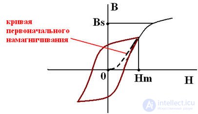
В случае переменного магнитного поля магнитная индукция изменяется по гистерезисной зависимости 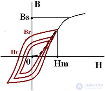
Bs - магнитная индукция насыщения
Br - остаточная магнитная индукция (Н=0)
Hm - амплитуда напряженности магнитного поля
Hc - коэрцитивная сила (В=0)
Нс<4кА/м- материал магнито-мягкий
Нс>4кА/м-материал магнито-твердый
Магнито-мягкие материалы
С округлой петлей гистерезиса 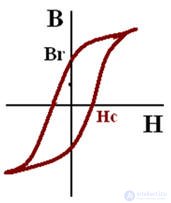
С прямоугольной петлей гистерезиса 
С линейной зависимостью В(Н) 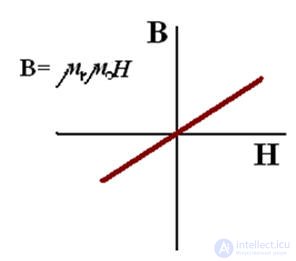
Магнитопроводы из ферромагнитов с прямоугольным гистерезисом применяют в оперативной памяти цифровых электронных вычислительных машин, устройств автоматики, магнитных усилителях.
Магнитопроводы из ферромагнитов с округлым гистерезисом применяют для изготовления электрических машин.
Магнитопроводы из ферромагнитов с линейными свойствами применяют для изготовления индуктивных катушек в радиотехнике (антенных устройствах, передатчиках и т.д.)
Ферромагнитный сердечник усиливает магнитное поле, возбуждаемое обмоткой , и увеличивает ЭДС самоиндукции. Для уменьшения м.д.с. F и следовательно тока I, необходимых для создания Ф, катушки снабжают магнитопроводом (сердечником). 
Магнитодиэлектрики и ферриты
В радиотехнике используют сигналы высокой частоты и сердечники для индуктивных катушек изготавливают из магнитодиэлектриков или из ферритов.
Магнитодиэлектрики – материалы, полученные при смешивании порошка магнетика, железа или пермаллоя с диэлектриком. Смесь формуют и запекают. Так как каждую крупинку обволакивает пленка из диэлектрика, такие сердечники не насыщаются
µ = 1-100.
Ферриты – материалы, которые изготавливают из окислов меди или цинка и окислов железа и никеля. По своим электрическим свойствам ферриты являются полупроводниками и могут насыщаться.
Нс=10 А/м.
µ=1-1000
Магнитотвердые материалы
Магнитотвердые материалы – углеродистые стали, сплавы магнико.
Постоянные магниты - сплавы железа с алюминием, никелем и кобальтом – альнико
Разновидность магнитных цепей
Неразветвленные цепи (тороиды, дроссель).
Разветвленные цепи (симметричные I1•W1=I2•W2, несимметричные I1•W1#I2•W2).
(трансформаторы и т.п.) 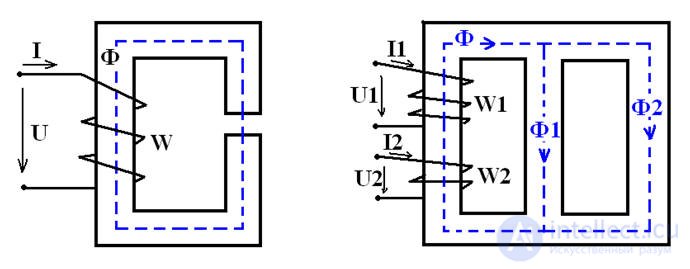
Рис 6
В параллельных ветвях разветвленной магнитной цепи с Н1 и Н2 и средними линиями l1 и l2 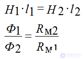
Законы Кирхгофа для магнитных цепей
1-ый закон – алгебраическая сумма магнитных потоков в любом узле магнитной цепи равна 0. 
2-ой закон – алгебраическая сумма падений магнитного напряжения Uм =Н∙l вдоль любого замкнутого контура равна алгебраической сумме м.д.с.. 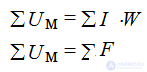
ЭМУ с постоянными магнитными потоками 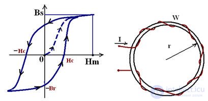
Рис 7
Тороид с толстыми стенками 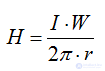
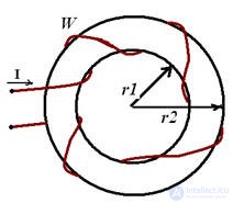
Рис 8
Абсолютная магнитная проницаемость и индукция 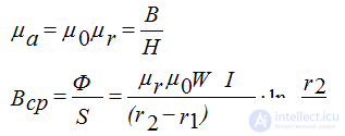
Throttle
Индуктивную катушку со стальным магнитопроводом называют дросселем. Это электромагнитное устройство, в котором катушка регулирует ток. 
Чем выше L, тем меньше ток I, следовательно можно изменять количество витков катушки 
1 – обмотка с числом витков W
2 – магнитный поток Ф
l1 – воздушный зазор
Если приложить к обмотке U, то потечёт I, который наведёт в магнитопроводе магнитный поток Ф, который индуцирует в обмотке ЭДС самоиндукции Е.
Действительное значение: 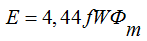
При синусоидальном напряжении на зажимах обмотки индуцированная ЭДС тоже синусоидальная, следовательно если пренебречь потерями напряжения на обмотке, то 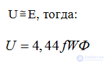
Фm=BmS,
S - площадь поперечного сечения магнитопровода
Bm – максимальное значение индукции 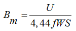
Индуктивность L рабочей обмотки зависит от магнитного сопротивления магнитной цепи 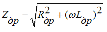
Rдр – сопротивление провода обмотки
Применение: в эл. машинах, в индуктивных датчиках и фильтрах выпрямителей
Трансформатор
Трансформатор – преобразователь электромагнитной индукции электрической энергии тока одной величины напряжения в электрическую энергию другой величины напряжения при f =const.
Трансформатор – повышает безопасность эксплуатации оборудования.
Один из самых распространенных видов электротехнического оборудования. Трансформатор рассчитан на определенную частоту.
Номинальная работа трансформатора при номинальных значениях токов и напряжений, которые указываются на щитке трансформатора и в его паспорте.
Трансформаторы бывают:
1. Однофазные
Понижающие и повышающие. Для питания тиристорных выпрямителей. Миниатюрные. Измерительные.
2. Трехфазные
Повышающие и понижающие.
С помощью повышающих трансформаторов доводят до напряжения 10-100 кВ и передают на подстанции. На станциях напряжение понижают с помощью понижающих трансформаторов. Для получения низких напряжений 380, 220, 127 В и распределяют по приемникам.
Application:
Силовые разделяющие трансформаторы, преобразующие Uсети в рабочее(трёхфазные).
Однофазные и трёхфазные для питания тиристорных выпрямителей двигателей постоянного тока.
Для питания ферроплавительных и плазменных печей. Повышающие трансформаторы с 380 В до 50 кВ – для питания электронно-лучевых установок и электрофильтров.
Миниатюрные трансформаторы в вычислительных машинах.
Измерительные трансформаторы U и I, для расширения пределов измерения приборов, для безопасности в цепях высокого напряжения.
Конструкция трансформатора.
Состоит из 2х обмоток – первичной, к которой подключают источник питания и вторичной, к которой подключают приёмники и стального магнитопровода. Если вторичных обмоток много, то трансформатор называют многообмоноточным.
Конструкция трансформатора зависит от габаритов, которые определяются номинальной мощностью.
Sном = UномIном 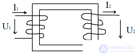
Причем, потерями принебрегаем, тогда: 
Схема замещения трансформатора:
В соответствии с принципом действия и конструкцией трансформатора следует, что его первичная и вторичная обмотки изолированы друг от друга и между ними существует только электромагнитная связь. Между токами первичным и вторичным отсутствует гальваническая связь, это усложняет процесс анализа работы трансформатора. Для упрощения анализа трансформатора используют схему замещения приведённого трансформатора. Реальный трансформатор имеет параметры: Мощность Р1, Q1, S1, cosφ2, U1, I1, R1, X1, E1 – эти параметры первичной цепи неизменны. Приводятся только параметры вторичной обмотки: 
Приводятся вторичные параметры к числу витков первичной обмотки и напряжению U1
Полная схема замещения трансформатора 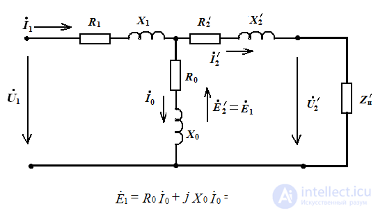
- R0 - активное сопротивление первичной обмотки
- R1 - активное сопротивление обусловленное магнитными потерями мощности в магнитопроводе
- R2ʹ - приведенное активное сопротивление вторичной обмотки
- X1 - индуктивное сопротивление первичной обмотки, обусловленное потоками рассеяния
- X0 - индуктивное сопротивление, обусловленное основным магнитным потоком
- X2ʹ - приведенное индуктивное сопротивление вторичной обмотки
n - коэффициент трансформации
Режим холостого хода (х.х.)
Режим при котором первичная обмотка включена на номинальное напряжение U1НОМ, а вторичная обмотка разомкнута. 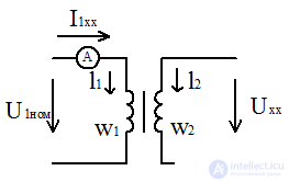
w1,w2 – число витков в 1 и 2 обмотках соответственно.
Режим работы трансформатора в х.х. такой же, как в индукционной катушке.
Ток в первичной обмотке i1X создаёт МДС  , которая вызывает магнитный поток Ф(t). Он пронизывает первичную и вторичную обмотки трансформатора.
Ф навозит в обмотке ЭДС е1 и е2 – действительные значения
E1= 4,44fw1Фm,
E2=4,44fw2Фm.
коэффициент трансформации 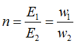
В режиме х.х. E1~U1ном, E2~U2х, тогда 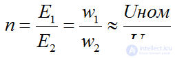
если n>1 то трансформатор понижающий
если n<1 то трансформатор повышающий
Активная мощность потребления трансформатора в режиме х.х.
Ртр хх=Рм+Рэ1 – общая формула
затрачивается на потери в магнитопроводе и электрические потери в первичной обмотке трансформатора, т.е.
Рэ1=0 т.к. Iхх→0 => Ртр хх=Рм
Определяется коэффициент мощности магнитных потерь и полное сопротивление трансформатора: 
Режим нагрузки 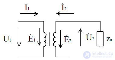
Нагрузка:
Electric motors
Осветительные устройства
Выпрямители т.д.
Из опыта с нагрузкой определяется:
P2=U2I2
коэффициент нагрузки 
КПД 
Короткое замыкание трансформатора
В условиях эксплуатации режим к.з. создаёт аварийный режим, т.к. вторичный ток как и первичный возрастает в несколько десятков раз по сравнению с номинальным, следовательно ставят защиту, которая при к.з. автоматически отключает трансформатор от сети.
Исключения составляют измерительные трансформаторы тока, специальные печные трансформаторы, которые выдерживают кратковременные к.з. Длительность к.з. < 10-12 сек. Электропечные трансформаторы для дуговых установок рассчитывают на 3х кратную перегрузку.
При опыте к.з. определяются параметры короткой сети.
Вторичную обмотку замыкают накоротко. 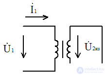
На вход подают 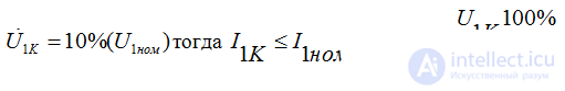
При опыте к.з., мощность потреб***яемая трансформатором идёт на нагрев обмоток трансформатора, т.е. равна электрическим потерям РЭ в проводах обмоток. 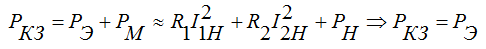
The main parameters of the transformer
Nominal:
Primary voltage U1
Secondary voltage U2
Primary current I1
Secondary current I2
Transformation ratio
Full power SH
Power factor 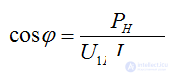
Efficiency 
Load factor 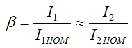
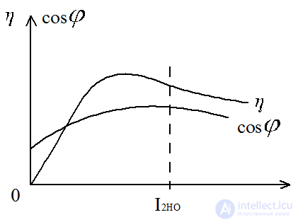
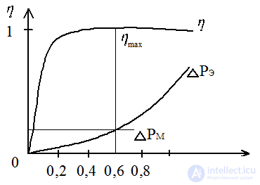
Optimal load factor 
Transformer external characteristic
The dependence of the secondary voltage U2 on the current I2 at a fixed voltage U1, with cosφ = const 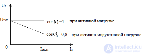
The higher the load current I2, the lower the voltage U2, but within 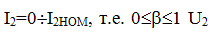 changes, that is, below a few%.
Load characteristics 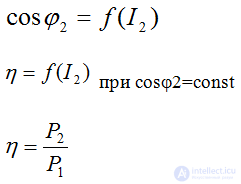
P2 - active power given to the consumer,
P1 - active power received from the network source  low-power transformers
electric furnace transformers have 
from the experience with the load 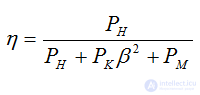
 - electrical losses
  - magnetic losses depend on the load factor
Electromagnetic field theory
Electromagnetic processes in all electrical devices can be considered from the point of view of field theory, since many laws that are used in the calculation of the circuits of these devices are based on this theory.
These laws include 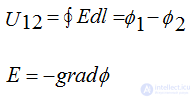
The last expression is applicable if the electric field is related to electric charges by the Coulomb law
Grad gradient of potential φ is a vector, any component of which is equal to the rate of increase of potential in the direction of the coordinate; the direction of the gradient φ is the direction of the most rapid increase of φ. 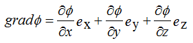
In practical electrical engineering, almost all sections are related to field theory.
In radio engineering - the propagation and reception of electromagnetic waves.
In electric cars.
Insulation technology.
High voltage technology.
Electromagnetic phenomena can be described from the point of view of field theory, and quantitative relationships and particular laws can be found from a small number of equations.
These equations are called Maxwell equations.
Maxwell equations in integral form
1st Maxwell's equation is the law of total current 
contour integral over a closed line l from H passing through a closed surface
H - magnetic field strength
H = B / μ0, in the case of vacuum,
J = σ • E - Ohm's law
Jп = J + Jcm is the total current, as the sum of the transfer current of electric charges and the displacement current, the density of which is:
where D = εε0 • E is the electric charge shift
Designations
σ - electrical conductivity (shows friction, with the passage of charges)
Q - charge in volume
ψ - electric displacement vector flux
ρ is the average charge density
P - electric polarization
M - magnetization
The simplest case of the 1st equation 
2nd Maxwell Equation - Electromagnetic Induction Law
emf induced in a closed loop by a varying magnetic field is equal to the rate of decrease of the magnetic flux coupled to the circuit in question. 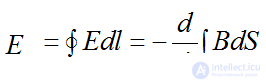
3rd equation for the electrostatic field (Gauss theorem)
The flux of the vector of electrical displacement, coming out through a closed surface, is equal to the charge contained inside this surface. The charge expresses the volume integral of its density over the volume of the surface under consideration. 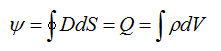
For magnetic field
The magnetic flux through any closed surface is zero.
B = μμ0 • H 
Maxwell equations in differential form
Divergence (divergence) of the force vector F 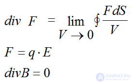
Any charge q being in an electric field of strength E is experiencing a force F.
Rotor (vortex of force vector F) lines of force 
1st Maxwell's equation 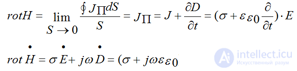
Differentiation is replaced by jω in the case of a simple harmonic signal
2nd Maxwell's equation the case of magnetic permeability 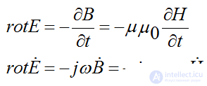
3rd equation Gauss equation for electrostatic field
The divergence of the electric displacement vector is equal to the electric charge density 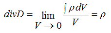
in case of constant permeability: 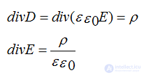
Relationship between vectors
J = σ • E - Ohm's law
D = ε0 • E + P
H = B / μ0 -M
Conductor with current divH = 0
Inside conductor rotH = J ≠ 0
There is no current in the outer region of the conductor. RotH = 0
Law of conservation of electricity
Let there be no dielectric and magnet in the electric field
P = 0 ε = 1 M = 0 μ = 1
the change in the electric field is accompanied by the same magnetic field as the movement of the charge 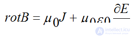
Constant field
rotB = μJ
With a changing field, this equation loses its meaning.
The current flowing out of any closed surface is equal to the decrease in the amount of electricity Q contained inside this surface. 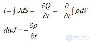
Corollaries of Maxwell's equations
A changing electric field is accompanied by a magnetic field - in the absence of current (charge movement), there must be a magnetic field whose vortex is equal to the rate of change of the electric field.
1. There is an electrical phenomenon without electricity.
2. There is a magnetic phenomenon without magnetism. 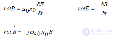
3. The existence of electromagnetic waves propagating at the speed of light
Electromagnetic waves
field of a wave traveling at the speed of light v = c 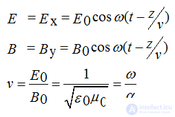
ε0 • Е - electric charge displacement В / μ0 - magnetic force 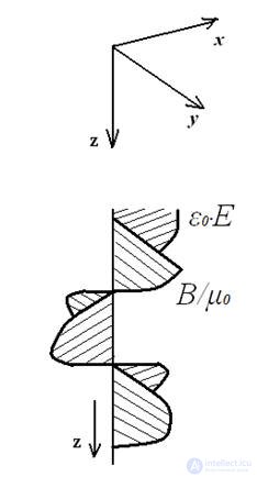
Chains with distributed parameters
At high voltages above 35 kV, at high frequencies above 50 Hz, in telecommunication engineering, with a significant length of transmission lines el. energy to neglect the currents of displacement and leakage through the garlands of insulators and corona is unacceptable, since the current in the wires has a different value in different sections of the line.
The current in the wires of the line causes a voltage drop in the active resistance of the wires and creates an alternating magnetic field, which in turn induces self-induction along the entire EMF line. Therefore, the voltage between the wires is also not constant along the line.
In order to take into account the change in current and voltage along the line, it is considered that each element of the line (segment) has R and L, between wires Y and C - this line is called a chain with distributed parameters.
If we assume that R and L, Y and C are uniformly distributed along the line evenly, which is an idealization, then such a line is called homogeneous. 
Figure 1 Homogeneous line
Homogeneous line parameters 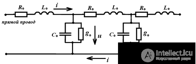
Ro is the resistance of the forward and reverse wires;
Lo is the inductance of the loop formed by the direct and return wires;
go - conductivity (leakage) between the wires;
Co is the capacitance between the wires, or between the wires and ground (working capacitance).
Differential equations based on Kirchhoff's laws 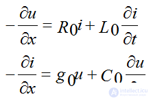
If the power source is sinusoidal in nature and in line steady state 
Instantaneous Voltage and Current 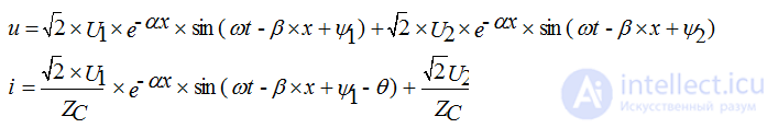
Ѳ - wave resistance argument 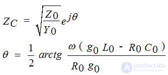
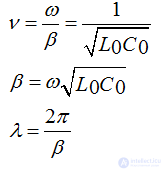
• Attenuation coefficient - α
• Phase ratio - β
• Wave propagation coefficient - γ
γ = α + jβ
• Characteristic or characteristic impedance - Zc
• Input resistance line Zin
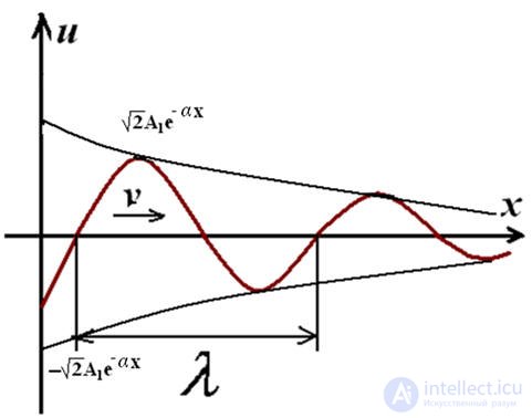
Expressions for voltage and current are expressions describing a traveling wave moving in the direction of increasing or decreasing coordinate X and decaying in the direction of the wave movement.
Forward and reverse waves are a convenient technique for decomposing the resulting current and line voltage. 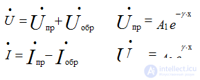
Solution of equations in hyperbolic functions
A1 and A2 - are determined if the boundary conditions are known
U1 and I1 values at the beginning of the line (for X = 0)
If we choose arbitrarily U1 and I1, then we are asked, depending on them and on the parameters of the line, the resistance at the end of the line Z2
at X = 0 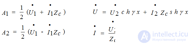
At a constant current ω = 0. There is no self-induction emf and bias currents between the wires. But there is an electric and magnetic field between the wires. 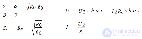
α - characterizes the attenuation of the amplitudes of the forward and reverse waves (Nep / km, dB / km)
β - characterizes the phase change of the wave depending on the x-point of the line (rad / km) 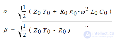
The resistance determines the currents of the forward and reverse waves at the corresponding voltages is called the wave Zc
The mean value of the Zc module for
overhead lines 300-400 ohms.
cable lines 50 ohm
In cable lines of strong current C0 is very large, L0 is very small, ε = 4-5, therefore the characteristic impedance is 6-8 times less than in overhead lines.
In lines with frequency ω = ∞ 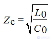
For air and cable lines g0, a negligible value, C0 is of great importance, therefore: 
Air and cable lines
Aerial wavelength 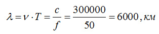
Input impedance line.
Concentrated resistance, which can replace the line with the load at its end. 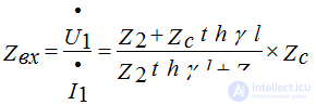
Idle 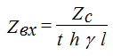
In short circuit mode 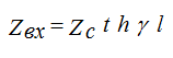
The reflection coefficient of the wave - in the line with the load a reverse wave occurs. This is taken into account when introducing a reflection coefficient ñ 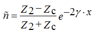
The reflection coefficient is determined in the places of the line, where there is heterogeneity, usually the beginning and the horses of the line. 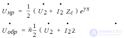
If the reflected wave does not occur, then such a load is called a consistent or load without reflections. In this case, the reflection coefficient is equal to 0. The absence of a reverse wave means that all the power carried by the direct wave to the end of the line is absorbed by the load.
Power transmitted on a consistent line is called natural or natural.
Natural power mode may occur in high voltage lines 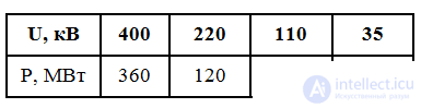
Efficiency 
Αl attenuation is measured in Nep or dB
1 nep - when the active power at the beginning of the line is more than the active power at the end of the line by e2 times.
Decibel decay 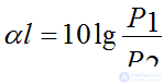
No distortion lines
The line in which the condition is met 
and the attenuation coefficient does not depend on the frequency and at the same time has a minimum value, is called a line without distortion.
Characteristic impedance does not depend on frequency 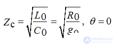
Phase velocity
Does not depend on frequency or at high frequencies 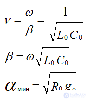
Line without distortion at matched load, voltage and current coincide in phase at any point of the line. The energy of the magnetic and electric fields at any given time are equal to each other. 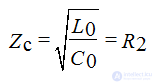
Cable lines without special devices are not suitable for transmission of speech, music over long distances.
The lines are suitable for transmission of speech, music over long distances, when the attenuation coefficient does not depend on the frequency or has a small value.
Lossless line
If we set equal to zero the resistance of the wires R0 and the leakage conductance between the wires g0, then we get a line without losses. (perfect line)
R0 = 0; g0 = 0; α = 0; 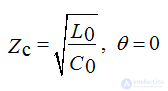
Phase speed for a two-wire line
Capacity and inductance of a unit of length of a line: 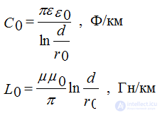
where r0 is the radius of the wire, d is the distance between the axes of the wires 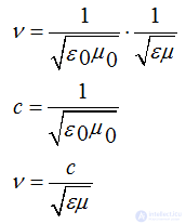
For overhead lines, ε = 1 and μ = 1; v = c
For cable lines ε> 1; v <c
The currents of the forward and reverse waves coincide in phase with the voltages.
Lossless Line Properties
Long quarter wavelength line 
Long half wavelength line: 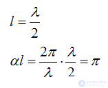
Standing waves
In the lossless line absorbed by the receiver, the active power is zero.
This is possible in the following cases:
When idle
Short circuit
With purely reactive load
A standing wave is a process resulting from the superposition of forward and reverse waves with the same amplitudes.
Idling
I2 = 0 Z2 = ∞ 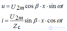
Equations of standing waves for instantaneous currents and voltages with ñ = 1
At any time at the end of the line X = 0 and at points spaced from the end of the line at distances 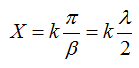
where k is an integer, when voltage peaks are obtained called antinodes, and current zeros, called nodes. Nodes and antinodes are always immobile.
The current is ahead of the voltage by 90 and vice versa. 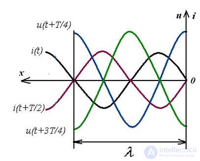
At the distance from the end of the line we have the opposite nodes of voltage and current antinodes. 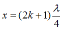
The input impedance is purely reactive and is determined by the wavelength (line) and frequency f. 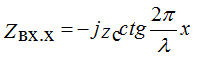
If x = 0 ÷ λ / 4 and x = λ / 2 ÷ 3λ / 4 line represents the capacitance.
If x = λ / 4 ÷ λ / 2 and x = 3λ / 4 ÷ λ, the line represents inductive resistance.
If x = 0, λ / 2, λ, etc. the line seems to be a parallel resonant circuit.
If x = λ / 4, 3λ / 4, etc. the line is represented as a sequential contour
Consistent load line
For matching it is necessary to have the shortest length for the line, i.e. instead of capacitance, choose an open line with a length of λ / 4, instead of inductive resistance, choose a short-circuited line with a length of λ / 4. 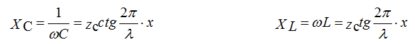
With a purely reactive load, there will also be standing waves in the line. Capacitive and inductive resistances can be replaced by open and short-circuited line segments. Only at the end of the line loaded on the reactance, there will be no antinodes or current and voltage nodes.
Lossless line loaded on resistive load 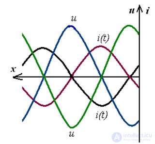
The equations for current and voltage at the end of the line contain two components 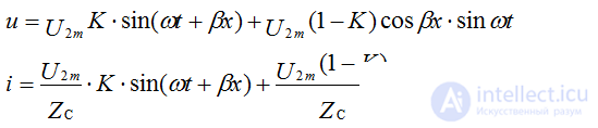
The first term traveling wave
Second term standing wave
If the line is not consistent with the load, i.e.K 1
in the line will be, and running, and standing waves.
If K = 0 or K = ∞, only standing waves will be in the line.
If K → 1, the traveling waves. When K = 1, there are no standing waves
Any exercises on the study of electrical engineering should begin with the study of lecture material and the corresponding section in the textbook. It is also necessary to learn the rules for compiling equations and properties of connections of elements of schemes.
Calculation of linear DC electric circuits
serial connection example 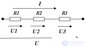
RACK = R1 + R2 + R3
I = E / R EQ
U = U1 + U2 + U3 = R1 • I + R2 • I + R3 • I = Rekv I
Task 1
It is necessary to measure the voltage of 100 V, a voltmeter of 10 V, with an internal resistance of 10 kΩ. What to do?
Add in series to the voltmeter resistor Rdob 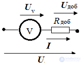
Payment 
Conclusion: a serial connection, as a voltage divider, can be used to extend the range of measurement of voltmeters
Parallel - serial connection
parallel connection. 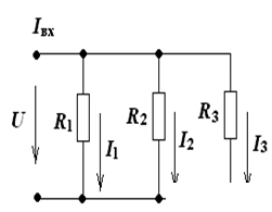
Iin = I1 + I2 + I3
I1 = U / R1 = UG1
I2 = U / R2 = UG2
I3 = U / R3 = UG3
Task
Determine equivalent resistance 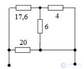
Considering this circuit, we see that the circuit has a series parallel circuit, where the resistors with resistances of 4 and 6 ohms are connected in parallel. Convert this area, we get 2.4 Ohms. Next, a 17.6 ohm resistor and a 2.4 ohm resistor are connected in series with 20 ohms, so we get 20 ohms. It remains parallel to 20 ohms and 20 ohms. The answer is equivalent to 10 ohms.
Decision 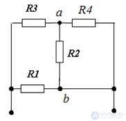
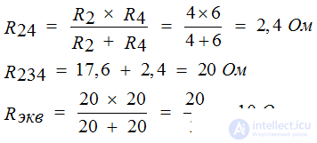
Task
Determine the equivalent resistance if R1 = R4 = R5 = 5 Ω R3 = R2 = 10 Ω 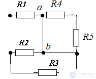
The plot with resistors R4 and R5 is shorted, therefore: 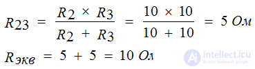
Equivalent Transformation Method
Task 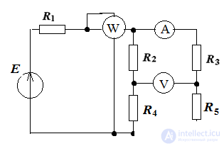
Determine the readings of the circuit devices in Fig. 1 if R1 = 5 Ω, R4 = 8 Ω, R5 = 4 Ω, R3 = 6 Ω, R2 = 2 Ω, E = 100 V. Calculation is carried out by the method of equivalent transformations
Decision:
we write the equation according to the laws of Kirchhoff to verify the calculation of currents 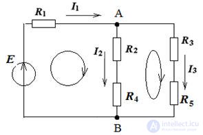
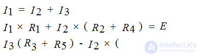
We turn the scheme, i.e. simplify the circuit and determine the equivalent resistance: 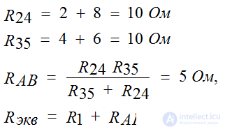
Determine the source current according to Ohm’s law 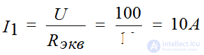
Determine the voltage between nodes A and B, then the currents I2 I3 
Determine the readings of devices:
The ammeter will show the current value I3 I3 = IA = 5 A
Voltmeter readings. Consider the contour of figure 2. 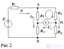
We write the equation according to the Kirchhoff law for the selected contour: 
Wattmeter readings: 
Задача метод контурных токов
Given:
R1 = R5 =10 Ом, R4 = R6 = 5 Ом, R3 = 25 Ом, R2 = 20 Ом, Е1 =100 В, Е2 =80 В, Е3 =50 В 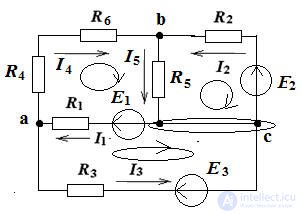
Определяем количество узлов, ветвей и независимых контуров: q = 3, p = 5, контуров 3. Составляем уравнения по законам Кирхгофа: уравнений по 1-ому закону Кирхгофа равно 2, а уравнений по 2-ому закону Кирхгофа равно 3. для узлов а и b. Для контуров выбираем обходы по часовой стрелке: 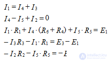
Так как три контура, то будет три контурных тока I11, I22, I33. Направления этих токов выбираем по часовой стрелке рис 3. Запишем настоящие токи через контурные:
I1 = I11 - I33, I2 = - I22, I3 = - I33, I4 = I11, I5 = I11- I22
Запишем уравнения по второму закону Кирхгофа для контурных уравнений в соответствии с правилами.
Правило: если ЭДС и ток имеют одинаковое направление с направлением обхода контура, то они берутся с «+», если нет, то с «–». 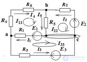
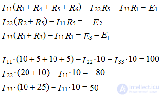
Решим систему уравнений математическим методом Гаусса или Крамера. 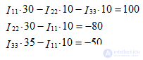
Решив систему, получаем значения контурных токов:
I11 = 2,48 А, I22 = - 1,84 А, I33 = - 0,72 А
Определим настоящие токи:
I1 = 3,2 А,
I2 = 1,84 А,
I3 = 0,72 А,
I4 = 2,48 А,
I5 = 4,32 А
Проверим правильность расчёта токов, подставив их в уравнения по законам Кирхгофа.
Составим уравнения для расчёта баланса мощностей: 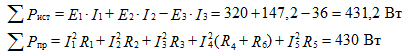
Из расчёта видно, что баланс мощностей сошёлся. Погрешность меньше 1%
Задача метод узловых потенциалов
Given: 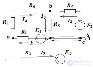
R1 = R5 =10 Ом, R4 = R6 = 5 Ом, R3 = 25 Ом, R2 = 20 Ом, Е1 =100 В, Е2 =80 В, Е3 =50 В
Определить токи в ветвях разными методами, составить и рассчитать баланс
мощностей
Решаем задачу методом узловых потенциалов
Составим уравнения 
Ток в любой ветви схемы можно найти по обобщённому закону Ома. Для этого необходимо определить потенциалы узлов схемы. Заземлим любой узел схемы φс = 0.
Решая систему уравнений, определяем потенциалы узлов φa φb
φa= 68 B φb = 43,2 B
По обобщенному закону Ома определяем токи в ветвях. Правило: ЭДС и напряжение берутся со знаком «+», если их направления совпадают с направлением тока, и со знаком «–» , если нет. 
Построение потенциальной диаграммы внешнего контура
Расчёт потенциалов и точек схемы
Пример расчета цепей с особенностями.
Особенностью является, наличие в схеме ветви с идеальной ЭДС
Given: 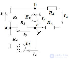
R1 ÷ R5 =10 Ом, Е1 = 30 В, Е2 = 60 В
Ток в любой ветви схемы можно найти по обобщённому закону Ома. Для этого необходимо определить потенциалы узлов схемы. Заземлим любой узел схемы φс = 0, тогда потенциал узла b равен значению E1 (если ЭДС направлен к узлу, то ЭДС берётся со знаком «+»). В данной схеме составляем одно уравнение для определения потенциала узла а.
При решении схем с особенностями заземляется узел к которой подсоединена ветвь с идеальной ЭДС. 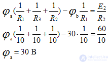
По обобщенному закону Ома определяем токи в ветвях. 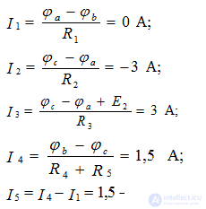
Пример метод двух узлов
Применяется в случае, когда схема содержит только два узла (параллельное соединение).
Algorithm:
Задаются положительные направления токов и напряжение между двумя узлами произвольно;
Уравнение для определения межузлового напряжения 
где G – проводимость ветви, J – источники тока;
Правило: G•E и J берутся со знаком «+», если Е и J направлены к узлу с большим потенциалом;
Токи схемы определяются по обобщенному закону Ома
Задача
Определить токи в ветвях методом двух узлов
Given:
R1 ÷ R3 =10 Ом, Е1 = 100 В, Е2 = 10 В 
Зададимся направлениями токов произвольно. Запишем уравнение для определения напряжения между узлами. Потенциал φa > φb и задаемся направлением напряжения от а к b.
Decision: 
Проверка по первому закону Кирхгофа: 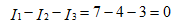
Метод эквивалентного генератора (двухполюсника)
Любой активный двухполюсник может быть заменен эквивалентным двухполюсником с параметрами Еэкв и Rэкв или Jэкв и Gэкв , режим работы схемы при этом не изменится
Задача 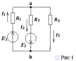
Определить токи в ветвях методом эквивалентного генератора в схеме рис 1
Given:
R1 ÷ R3 =10 Ом, Е1 = 100 В, Е2 = 10 В
Зададимся направлениями токов произвольно.
Определим первый ток
Разомкнуть ветвь с R1 для определения тока в первой ветви. 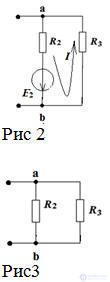
Определим эквивалентную ЭДС относительно разомкнутых зажимов рис 2 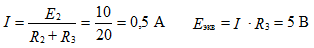
эквивалентное сопротивление рис 3 
Искомый ток I1 определяем по формуле 
Определим второй ток
Разомкнуть ветвь с R2 для определения тока во второй ветви. 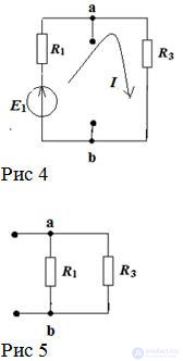
Определим эквивалентную ЭДС относительно разомкнутых зажимов рис 4 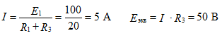
эквивалентное сопротивление рис 5 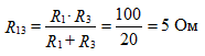
Искомый ток I2 определяем по формуле 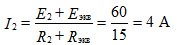
Определим третий ток
Разомкнуть ветвь с R3 для определения тока в третьей ветви. 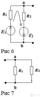
Определим эквивалентную ЭДС относительно разомкнутых зажимов рис 6 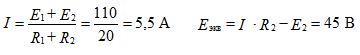
эквивалентное сопротивление рис 7 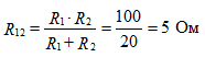
Искомый ток I3 определяем по формуле 
Пример расчета цепей с нелинейными элементами
Определить ток в цепи и напряжение на диодах вольтамперные характеристики (ВАХ) которых представлены на рис 8, если Uвх = 2,5 В, Rн = 25 Ом
Given: 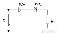
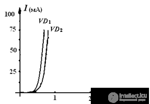
Рис 8
Решение: построим суммарную ВАХ диодов и
«опрокинутую» вольтамперную характеристику
нагрузочного резистора рис 9.
U = U1 + U2 + I•Rн
хх: U12 = U = 2,5 В
кз: Iкз = U/Rн = 2,5/25 = 100 мА 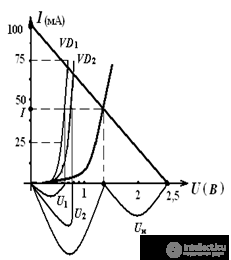
Fig.9
Answer: U1 = 0.6 V, U2 = 0.7 V, Un = 1.2 V, I = 45 mA
Для схемы на рис 10, стабилитрон имеет параметры:
Ust = 20 V, Ist min = 1 mA, Rdif = 40 Ohm, Ist max = 71 mA.
Determine the current I in the circuit in a graphical way, if In = 20 mA: 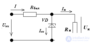
Decision:
I = Ist + In
Строим ВАХ стабилитрона по трём точкам 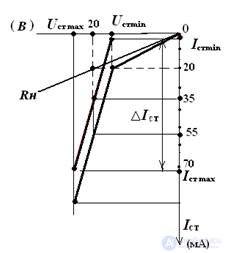
Рис.11
∆Ist = Ist max - Ist min = 71 - 1 = 70 mA
∆ Ust = ∆Ist • Rdif = 0.07 • 40 = 2.8 V
Ust min = Ust - ∆Ust / 2 = 18.6 V
Ust max = Ust + ∆Ust / 2 = 21.4 V
ВАХ резистора. We summarize the CVC-ki. Графически определяем ток неразветвленного участка цепи рис 11.
I = 55 mA
Перевод комплексных чисел
Перевести заданный во временной форме ток i(t)=141 sin(ɷt+90°) в комплексную форму: показательную и алгебраическую.
Decision:
амплитудное значение тока Im= 141 A
+90° – начальная фаза тока.
Запишем комплексный ток в показательной форме:
Комплексный ток амплитуды 
комплекс действующего значения тока 
В алгебраическую форму переводим используя формулу Эйлера 
Task 2
Задано напряжение в алгебраической форме 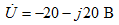
Перевести во временную форму.
Decision:
рассмотрим вектор напряжения на комплексной плоскости 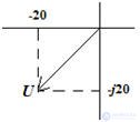
Получается, что вектор находится в третьей четверти комплексной плоскости. Это означает, что начальная фаза угла от 180° до 270°, т.е. к полученному углу прибавляем 180° 
Значение модуля напряжения определяем по теореме Пифагора 
Ответ: u(t)=40 sin(ɷt+225°)
Пример построения качественных векторных диаграмм
Task 3
Построить качественную векторную диаграмму.
Построение проводим, используя свойства элементов. Первым строится вектор тока, затем вектора напряжений. 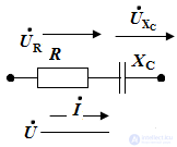

Задача 4
Построить качественную векторную диаграмму.
Построение проводим, используя свойства элементов. 
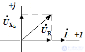
Задача 5
Построить качественную векторную диаграмму для цепи, при условии, если XL>XC.
Построение проводим, используя свойства элементов. 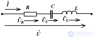
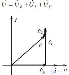
Task
В последовательной цепи определить показания приборов, составить и рассчитать баланс мощностей, определить коэффициент мощности, построить топографическую векторную диаграмму.
R1 = 10 Ом
R2 = 20 Ом
C = 31,8 мкФ
L = 0,127 Гн
f = 50 Гц 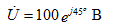
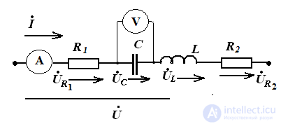
Decision:
one). Определим полные комплексные сопротивления реактивных элементов 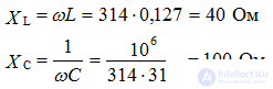
2). Переведем в алгебраическую форму напряжение источника 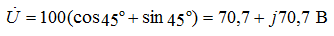
3). Определим эквивалентное сопротивление цепи 
Схема имеет активно-емкостной характер
four). Определим ток в цепи 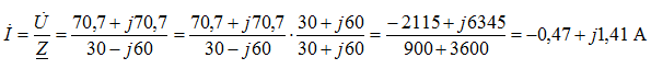
five). Амперметр покажет действующее значение тока 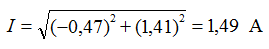
6). Определим показание вольтметра, действующее значение напряжения на конденсаторе 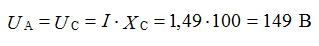
7). Определим мощности источника и приёмников 
Мощность приёмников 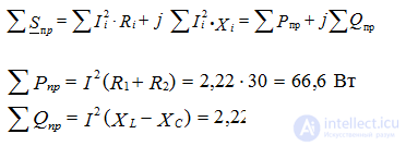
Из расчетов видно, что баланс сходится с погрешностью меньше процента 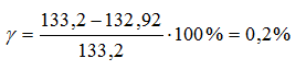
8). Определим коэффициент мощности 
9) построение топографической векторной диаграммы
Определим напряжения на элементах цепи 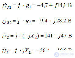
Выбор масштаба по току 2 см – 1 А; по напряжению 2см – 50 В
Правило построения векторной диаграммы, при последовательном включении элементов:
строим вектор тока
строим вектора напряжений
складываем вектора напряжений по правилу параллелограмма. 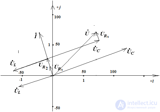
пример параллельное соединение
Определить токи в ветвях.
Given: 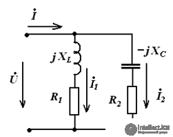
R1 = 10 Ом
R2 = 10 Ом
f = 50 Гц 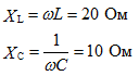
Decision:
3 ветви, 2 узла.
Токи определяем по закону Ома. Запишем полные сопротивления ветвей: 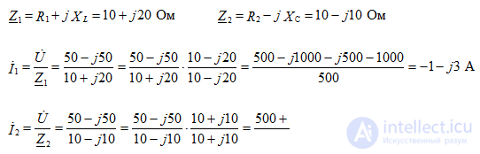
Общий ток определяем по первому закону Кирхгофа 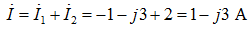
Vector diagram 
Task 
E = Uo + Um•sin(ωt + 45), Uo = 45 B, U = 39 B,
R1= R2 =50 Ом, L= 0,127 Гн, C= 3,18 мкФ
Определить Uc, I2
Решение
по постоянной составляющей
Е1 = Uo = 45 B I2 = Uo/R1 = 0,9 A I3 = 0 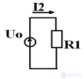
По переменной составляющей XL= 40, Ом Xc = 1000 Ом 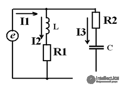
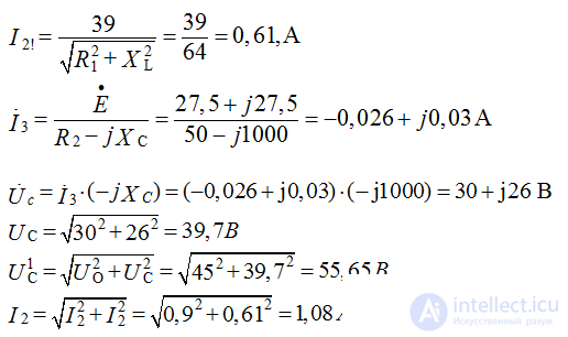
Пример резонанс напряжений
Определить сопротивления всех элементов и напряжение на резисторе. В цепи резонанс напряжений.
Given: 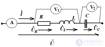
Амперметр показывает 2 А.
Вольтметры V1 = 80 В; V2 = 40 В
Decision: 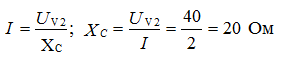
в цепи резонанс, значит из условия резонанса ХL = ХC = 20 Ом 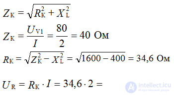
Резонанс токов
Определить значение емкости конденсатора, при котором возможен резонанс токов. Построить векторную диаграмму.
Given: 
R1 = 40 Ом
R2 = 10 Ом
f = 50 Гц 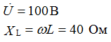
Decision: 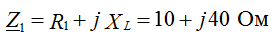
Условие резонанса токов: 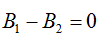
Определим значение проводимостей ветвей: 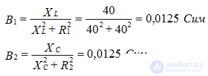
Решая квадратное уравнение, получаем два положительных корня со значениями
реактивного сопротивления Хс1 = 78,7 ; Хс2 = 1,25 Ом
выберем одно значение Хс2 = 1,25 Ом и проведем расчет тока: 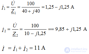
Построение векторной диаграммы 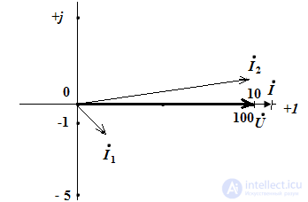
Построение диаграмм смешанного соединения
Задача 3 Построить качественную векторную диаграмму.
Построение проводим, используя свойства элементов. 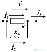
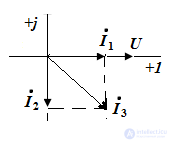
Задача 4 Построить качественную векторную диаграмму. Построение проводим, используя свойства элементов.
При построении векторной диаграммы смешанного соединения, сначала строим векторную диаграмму параллельного соединения, затем последовательного. 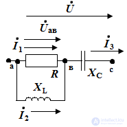

Расчет цепей при периодических несинусоидальных входных воздействиях.
Task 1
Определить ёмкость конденсатора, если его сопротивление на третьей гармонике равно 500 Ом.
Decision:
сопротивление конденсатора XС = 1/3ɷС = 500 Ом
С = 1/ XС ∙3ɷ = 1/500∙3∙314 =2, 12 мкФ
Task 2
Определить сопротивление катушки, при сигнале с пятой гармоникой, если при первой гармонике
XL = 5 Ом.
XL5 = 5∙ ɷ∙L = 25 Ом
Task 3
Определить коэффициент искажений и коэффициент гармоник, если на вход устройства подан сигнал: 
Решение: рассчитаем действующее значение напряжения источника 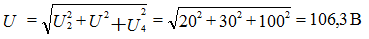
U1 = 0
КИ = U1/U=0
Коэффициент гармоник КГ = Uг/U
действующее значение высших гармоник 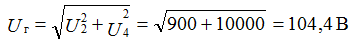
КГ = Uг/U =104, 4/106,3=0,928
Задача 4
Определить значения: U1, I2 
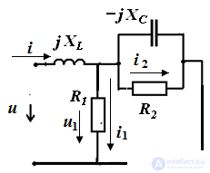
Given: 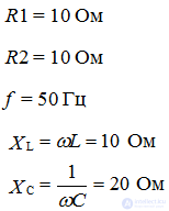
Расчет проводим методом наложения (суперпозиций).
1. Расчет по постоянной составляющей U = 20 B
Схема приобретает вид 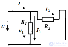
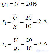
2. Расчет по первой гармонике 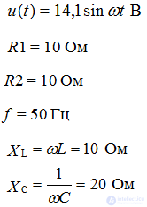
Decision 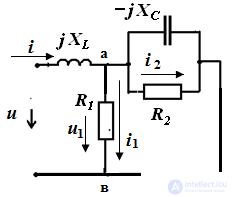
4 ветви, два узла
решать можно любым методом: эквивалентных преобразований, двух узлов
Решаем методом эквивалентных преобразований.
Найдем эквивалентное сопротивление: 
Действующее значение входного напряжения: 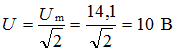
Комплексное напряжение 
Определяем ток источника: 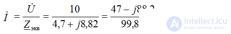
Определяем напряжение между узлами «ав» 
Действующее значение напряжения: 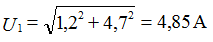
Определяем токи в ветвях: 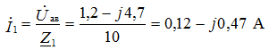
Действующее значение тока: 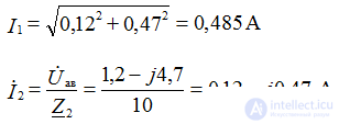
Действующее значение тока: 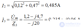
Действующее значение тока: 
3. Расчет по второй гармонике 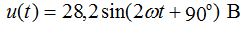
Комплексное напряжение 
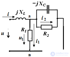
Decision
4 ветви, два узла
решать можно любым методом: эквивалентных преобразований, двух узлов
Пересчет значений реактивных сопротивлений 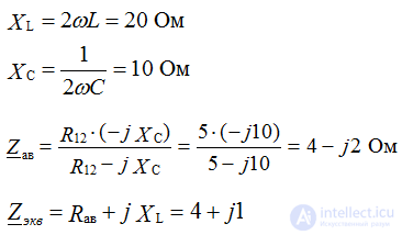
Действующее значение входного напряжения: 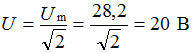
Определяем ток источника: 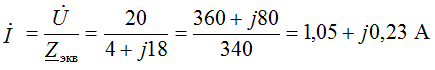
Определяем напряжение между узлами «ав» 
Действующее значение напряжения: 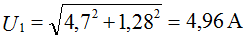
Определяем токи в ветвях: 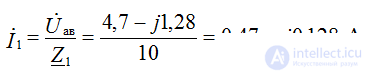
Действующее значение тока: 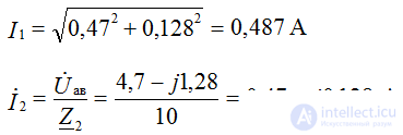
Действующее значение тока: 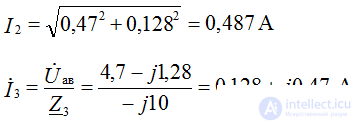
Действующее значение тока: 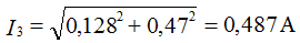
4. Итоговые расчеты. Определяем итоговые действующие значения: 
Приемник включен в четырехпроводную сеть звездой
Дано 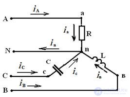
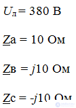
Определить ток в нейтральном проводе
Расчет фазных и линейных напряжений цепи 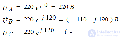
Расчет фазных токов в приемниках: 
Расчет тока в нейтральном проводе: 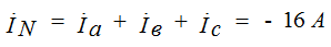
Обрыв нейтрального провода
Дано
обрыв нейтрального провода 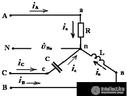
Uл = 380 В
Zа = 10 Ом
Zв = j10 Ом
Zс = -j10 Ом
Определить токи в фазах приёмника
Расчет фазных напряжений источника 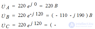
Расчет напряжения смещения нейтрали 
Расчет напряжений на фазах приёмника 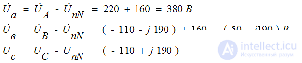
Расчет токов в фазах приёмника 
Сумма токов равна 0
Пример включения треугольником
Дано
Определить токи в фазах приёмника и в линиях
Фазные напряжения приемника равны соответствующим линейным напряжениям источника питания :
фазные токи:
Токи в фазах определяются по закону Ома:
Линейные токи определяются по фазным токам по первому закону Кирхгофа:
Сумма линейных токов равна 0
асчет переходных процессов в электрических цепях классическим методом
Task 1 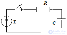
Построить переходной процесс при замыкании ключа.
Е = 10 В, С = 10 мкФ, R = 1 кОм
τ = RC = 0,01сек - постоянная времени зарядки конденсатора
Uс пер = Uс уст + Uc cв Uc уст = E = 10 В 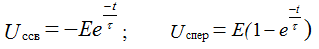
переходной процесс проходит по экспоненциальному закону.
τ- постоянная времени, в течении которого свободная составляющая процесса уменьшается в  раз по сравнению с начальным условием.
рассчитаем несколько характерных точек:
t = τ Uс пер1 = 10(1 -1/2,7) = 6,3 B
t = 2τ Uс пер2 = 10(1 -1/7,29) = 8,63 B
t =3 τ Uс пер3 = 10(1 -1/19,863) = 9,5 B
t =4 τ Uс пер4 = 10(1 -1/53,14) = 9,85 B
t =5 τ Uс пер5 = 10(1 -1/143,5) = 9,9 B 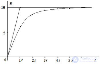
Task 2 
Построить переходной процесс при размыкании ключа.
Начальные условия Uc = Е = 10 В, С = 10 мкФ, R = 1 кОм
τ = RC = 0,01сек - постоянная времени зарядки конденсатора
Постоянная времени, в течении которого свободная составляющая процесса уменьшается в  раз по сравнению с начальным условием.
Uс пер = Uс уст + Uc cв Uc уст = 0 В
Uс пер = Uс св = переходной процесс проходит по экспоненциальному закону.
рассчитаем несколько характерных точек:
t = τ Uс пер1 = 10/2,7= 3,7 B
t = 2τ Uс пер2 = 10/7,29 = 1,37 B
t =3 τ Uс пер3 = 10/19,863 = 0,5 B
t =4 τ Uс пер4 = 10/53,14 = 0,15 B
t =5 τ Uс пер5 = 10/143,5 = 0,1 B 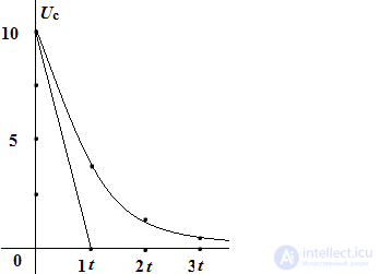
Task 3 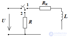
В схеме индуктивная катушка отключается от источника постоянного напряжения и замыкается на резистор
U = 110 В, L = 5 Гн Rк = 4 Ом, R = 6 Ом
Найти ток в катушке при t = 1 сек, её после отключения от источника и напряжение на R в начальный момент после коммутации
Решение когда источник подключен к катушке (положение ключа 1) ток в цепи определяется по закону Ома I = U/Rк =110/4 = 27,5 А
После коммутации, т.е. переключение ключа (положение ключа 2) электрическое состояние цепи описывается уравнением 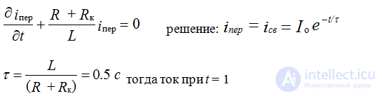
Напряжение UR = RI =27,5∙ 6 =165 B
Задача 4 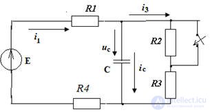
Дано: Е = 100 В; R1 = 20 Ом; R2 = 30 Ом; R3 = 10 Ом; R4= 40 Ом; C = 100 мкФ
Определить входной ток  и записать выражение
Decision
1. После замыкания ключа
Запишем уравнения по законам Кирхгофа 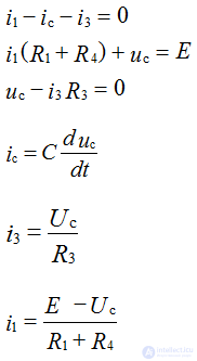
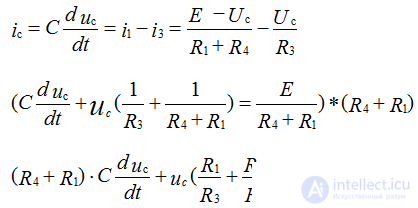
2. Расчет установившегося режима
Uс пер = Uс уст + Uc cв 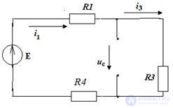
Составим уравнения для установившегося режима: 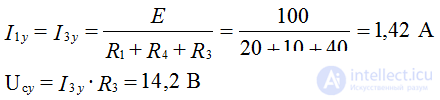
3. Решим одним из способов, определив параметры переходных характеристик через решение характеристического уравнения. Составим это уравнение: 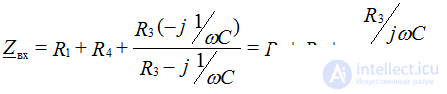
Заменим jɷ = p где p- корень характеристического уравнения 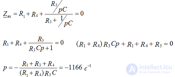
4. При t = 0: 
Uс (0+) = U(R2+R3) /(R1+R2+R3+R4)=40 B
Определяем значение А: 40 = 14,2 + AA= 25,8 B
Выражение напряжения на конденсаторе принимает вид: 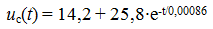
5. Записать выражение для входного тока 
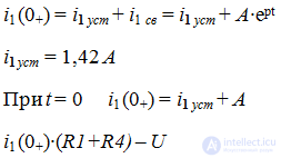

Определяем значение А: A = - 0,42
выражение для входного тока 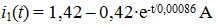
Задачи для самостоятельной подготовки
1. Синтезировать электрическую цепь из резисторов с номиналом 10 Ом, чтобы получилось эквивалентное 25 Ом.
Используем свойства последовательного и параллельного соединений 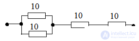
2. Определить Uab 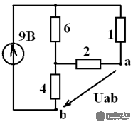
3. Определить показания приборов 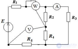
Дано: R1 = 2 Ом, R4 =3 Ом,
R5 = 1 Ом, R3 = 3 Ом, R2 =3 Ом,
Е = 75 В
4. Найти эквивалентное сопротивление, определить показания приборов. Определить мощность приемника и мощность источника. R1 = 10 Ом, R2 = 10 Ом, R3 = 20 Ом, U=30 В 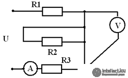
5. Упростить схему 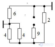
6.Определить ток и напряжение в нагрузке, напряжение на диодах (ВАХ и схема рис 12), если Uвх = 4, В Rн = 100, Ом. 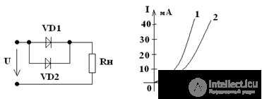

Comments
To leave a comment
Electrical Engineering, Circuit design
Terms: Electrical Engineering, Circuit design