3.5. Features of propagation of radio waves used in the GSM standard (decimeter waves (900 MHz, 1800 MHz, 1900 MHz))

As noted above, the GSM standard uses decimeter waves (900 MHz (k = 0.333 m), 1800 MHz (k = 0.167 m), 1900 MHz (k = 0.158 m)).

It should be noted that meter (VHF), decimeter and centimeter (UHF) electromagnetic waves from the ionized layers of the atmosphere are practically not reflected and not scattered in them and, therefore, like ionospheric waves cannot propagate. The waves of these ranges propagate mainly in the form of terrestrial waves (diffraction of such waves is poorly expressed) over short distances, and over large ones due to tropospheric scattering by inhomogeneities and, to a lesser extent, due to directional action of tropospheric waveguides.

UHF radio waves almost do not refract in the ionized layers of the atmosphere and freely penetrate them, that is, they propagate as direct waves and therefore are used in space communications; practically do not experience molecular absorption, absorption in hydrometeors (rain, snow), that is, in terrestrial conditions, decimeter waves can propagate only in a straight line within the line of sight.

Spreading in the line of sight, electromagnetic waves in cellular mobile communication systems experience numerous reflections from and absorption from surrounding objects. The multipath pattern shown in Fig. 3.12, indicates a superposition at the MS reception point of several, or more precisely, sets of signals coming in different paths and having different amplitudes, phases, propagation times, polarization planes, etc.

Due to this, the resulting signal at the receiving point changes dramatically and can be both above the average (median) level and lower, and signal fading resulting from the mutual compensation of signals due to the unfavorable combination of their amplitudes and phases can be quite deep. Distortion of the resulting signal occurs when the more or less in-phase components of signals with comparable amplitudes have such excellent path differences that the symbols of one signal are superimposed on the adjacent symbols of another, and inter-symbol interference occurs.

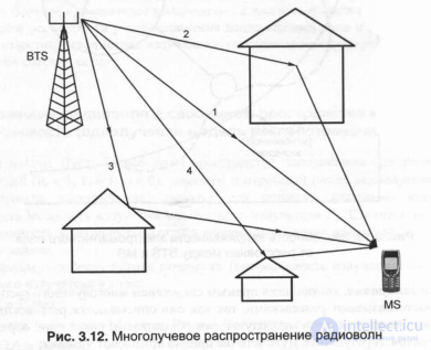
Fig. 3.12. Multipath propagation of radio waves

As shown in fig. 3.13, the dependence of the field strength on the distance between the BTS and MS is of a decreasing nature, with the field strength having both fast and slow fading relative to the average (median) value, that is, the average value is subject to decay, and the instantaneous values ​​are fading.

In the particular case for isotropic transmitting and receiving antennas BTS and MS, the ratio of the power at the reception point PR to the power at the transmission point Pr (in the absence of interference) can be written in the form:

Pr / Pt = (V4itrf = (c / 4n-rf) 2 (3.60)

where c = 3-10 m / s is the speed of electromagnetic waves in vacuum, / is the operating frequency, g is the distance between BTS and MS. With / = 900 MHz, g = 10 km: Pr / Pt = (2.6-10-6) 2,

Pr / Pt dB ~ -50 dB.

Thus, the attenuation value is inversely proportional to the square of the signal frequency and the square of the distance between the BTS and MS.

In the case of directional antennas, the gains of the transmitting and receiving antennas must be taken into account, which leads to the following formula:

PR / PT = GtGr (Wnfrf) (3.61)

where GT and Gr are the gains of the transmitting and receiving antennas.

Fluctuations of the levels (fading) of the received signal have two components - fast and slow.

Fast fading, which is a direct consequence of multipath propagation of radio waves, is often called Rayleigh, as they are described by Rayleigh distribution laws. Fading due to multipath due to signals reflected from external objects. As a result, the following conditions occur at the point of reception:

- several signals of the same type shifted in phase are added so that the resulting signal is attenuated;

- with the same level of the main and reflected signals, but their antiphase nature, the resulting signal is close to zero, which causes communication interruption.

The range of changes in the signal level during fast fading can reach 40 dB, of which approximately 10 dB is the excess over the average level and 30 dB are dips below the average level, and deep dips are less common than less deep ones. With a fixed MS mobile station, the intensity of the received signal remains almost unchanged. When the MS moves, the frequency of fluctuations in space is about the half-wave V2, that is, about 16.5 cm (at a frequency of 900 MHz).

The period of fluctuations depends on the speed of movement of MS, for example, at a speed of V = 50 km / h, the period of fluctuations of Tf is 10 ms, and at V = 100 km / h it is Tf ~ 5 ms.

The frequency of fading depth (30 ... 10) dB at a speed of V-50 km / h is 5 ... 50 dips per second, respectively, and the average duration of fading is below (30 ... 10) dB at a speed of V = 50 km / h - about (0.2. .2) ms.

Slow fading is caused by the shadow effect, which is caused by various obstacles (buildings, woodlands, mountains, etc.) that violate the direct visibility between the BTS and MS. Slow fading obeys the log-normal distribution law. The intensity of slow fading does not exceed (5 ... 10) dB, and their frequency corresponds to the displacement of MS by tens of meters. In fact, slow fading is a change in the average level of the signal as the MS moves, on which fast fading is superimposed due to multipath.

To combat fast fading in the GSM standard, jumps in frequency, i.e. spectrum expansion, are used, while equalizers — adaptive filters — are used to reduce intersymbol distortions. To combat the effects of multipath propagation, namely, to eliminate errors caused both by signal fading and intersymbol interference, noise-resistant channel coding is used: block and convolutional coding, as well as interleaving.

Consider the features of the propagation of decimeter waves and the calculation of the fields at the points of reception with known radiation parameters and the distance between the transmitter and receiver for the case of a cellular network.

Radio wave propagation in free space within the direct line of sight (single-beam propagation model)

Formulation of the problem. Let an isotropic (omni, omnidirectional) emitter (for example, an electric dipole), for which the radiation pattern F (cp) = 1, is placed in a free space filled with a homogeneous non-absorbing medium (| yag = 1, ε = 1, a = 0). Let the radiation power of the isotropic radiator Pr. The task is to determine the electric field intensity at an arbitrary point of reception M.

The solution of the problem.

1. Determine the power flux density (radiation intensity) at a distance r from an isotropic radiator in the form:
n = Pi / S = Pi / 4nr2. (3.62)

2. Considering that at the point M, the Umov-Poynting vector will be defined as П = E2J2Z0 = Pl / 4nr2, (3.63) where Ет is the amplitude of the electric field intensity, Z0 = 120л is the wave resistance of the medium

3. Find the magnitude of the amplitude of the electric field intensity Ет in the form: Ет = (60Р 01/2 / g, (3.64)), that is, this formula determines the magnitude of the amplitude of the electric field intensity at the receiving point, which in this case depends on the radiation power of the transmitting isotropic antenna Pr and distance r, to the point of reception.

Let's complicate the task, assuming that we replace the isotropic transmitting antenna with a directional one, that is, we define the power flux density in the form:

P = P, G, / 4ro-2, (3.65)

where G \ = r \\ Di is the gain of the transmitting antenna, d]! and Gi - efficiency and directivity of the directional antenna.

Then the expression (3.64) is written in the form:

Et = (60PxGx) mlr. (3.66)

In practice, they often use another type of formula (3.66):

Et = 245 (PiG1) 1/2 / r, (3.67)

where Pi (kBt), g (km), Et (mV / m).

Thus, the expressions obtained allow us to carry out estimates of the amplitude of tension at the point of reception Ет (г) for one electromagnetic beam (for the case when Ет is determined in the direction of the maximum of radiation).

In any direction:

adf) = £ l-de, f), (3.68)

where F (Q, f) is the transmitting antenna pattern.

In order to calculate the power at the output of the receiving antenna for this case, it is necessary to take into account that the receiving antenna is directional and has an effective aperture:

Ae 2 = C2X2 / 4l, (3.69)

where G2 is the gain of the receiving antenna.

We will carry out the following calculations:

- we find the power of the electromagnetic field at the point of reception in the form: Р2 = П'ЛЭ2 = (P1G1 / 4kt2) (G2X2 / 4k) = PlGlG2 Х2 / (4лг) 2; (3.70)

- taking into account the attenuation in the feeder of the receiving antenna, we determine the power at the receiver input in the form: pr = P2e ~ a <'= [Pfifii ^ 1 / (4lg) 2] e "a <', (3.71) where a and £ is the attenuation coefficient and the length of the feeder line.

Thus, the values ​​of E2 and Pr at the point of reception are determined by the radiation power of the transmitting antenna Pj, the directional properties of the transmitting and receiving antennas (Gx and G2), the distance between the transmitter and receiver, the working wavelength, and the feeder parameters.

If electromagnetic waves propagate in a dielectric medium with a dielectric constant gy (but in a lossless medium), then the value of wave resistance is equal to

Zb = 120l / (er) w (3.72)

and the values ​​of E2 and Pr will depend on the dielectric properties of the propagation medium (that is, on the dielectric constant of the medium g).

The propagation of radio waves in an environment with unchanged parameters.

Let's complicate the problem: let the radio waves propagate in an environment that is characterized by the attenuation function W (t) = const.

If the value of W is determined theoretically or experimentally, then for the single-beam model, the amplitude of the electric field and the signal power at the receiver input will be written: Et = 245 [(PlGi) m / r] W, (3.73)

P2 = [PiG1G27,2 / (4nr) 2] W2. (3.74)

Often use the formula for P2, written in decibels:

P2 = Fish + Gi + G2 + 20lgXi - 201g (4jtri) + W &. (3.75)

When Xi = ADO, T \ = g / go, ko = go = / m, P \ and P2 are written in dB relative to: Р0 = 1 W or 1 mW (RdB = 101g Р / Ро).

Consider the simplest numerical example.

Determine the power at the receiver input under the following conditions: transmitter power P \ t = Yu W, transmitter feeder attenuation - antenna: e "a /" 0.8, gain gains of the transmitting and receiving antennas G \ = G2 - 1.64, working length waves X = 33.3 cm, distance between BTS and MS g - 10 km, attenuation factor W »–20 dB, attenuation of the feeder of the receiving antenna: е_a /« 0.8.

Numerical calculation. Determine the power Rsch expressed in watts (3.71) and in decibels (3.72):

P2R = [Pfi & k, / (4lg) 2] I'2e ~ af ,, f'e ~ af2'f2 = 1.2Ю “10W, that is, Pw = -129.2 dBm.

If the sensitivity of the receiver is / 'min 1 (G12 W (that is, Rsch = -130 dBm)), the reception conditions will be difficult to achieve, since the signal level is close to sensitivity and below the allowable power margin (^ (3 ... 6) dB)

Determine the field strength at the receiving point under the above conditions and taking into account that the effective length of the receiving antenna is hg ** 6 cm, its radiation pattern is F2 (0) = sin0 (the beam arrives at 0 = 30 °) and the receiver sensitivity is Vmin = 0, l mV.

Numerical calculation. We use the formulas (3.54) and (3.73):

Y2 = hg-Em2 (F2 (e) / J2) = hg [6QP \ Gi) ll2 / r] WF (£ i) -e “° '5 (af | fi + af2'f2> (1Д / 2 ) = 106 10 6 V,

that is, V2 = 106 µV "U min = 0.1 µV, that is, the conditions of reception are provided.

Thus, the above examples allow in practice to carry out assessments of the conditions of sustainable mobile radio communications for the single-beam model, when they neglect the reflection from the earth, the influence of buildings, forests, etc.

Dual-beam model of radio wave propagation of decimeter range.

In fig. 3.14 shows the conditions for the rectilinear propagation of electromagnetic waves of the decimeter range.
Troposphere

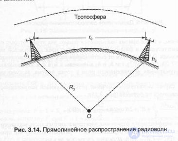
Fig. 3.14. Linear propagation of radio waves

In this case, the line-of-sight distance r0 is determined by the formula r0 = k $, R3) ([hi] 112 + [h2 \ m), km (3.74)

where hi and h2 are the heights of the transmitting and receiving antennas (expressed in meters), & (§, R3) is a coefficient depending on the conditions of atmospheric refraction (that is, on changes in the propagation path due to changes in the refractive index of the atmosphere) and on the earth radius R3.

propagation rate due to changes in the refractive index of the atmosphere) and on the radius of the earth R3.

If the refraction is absent or negligibly small, then the value of k (R3) = 3.57. Under normal atmospheric refraction, when the beam bends to the surface of the earth, the line-of-sight distance increases and the value of k (R, R) = 4.12. To increase the propagation distance of the decimeter wave band, transmitting antennas are usually raised to a certain height, for example, for antennas of BTS base stations - hi = 20 ... 100 m, for television antennas - hi- 40 ... 400 m, for antennas of radio relay communication lines - hi = (20 ... 80) m. The heights of raising the receiving antennas vary widely (from 2 to 80 m). In mobile communication systems, the elevation height of receiving antennas ranges from 1 m to 3 m.

To determine the field strength at the reception point for a given transmit power of the transmitting antenna Pi, its gain Gb of the elevation height hi and the distance r to the reception point, proceed from the following assumptions: 3.15 two beams are shown that propagate from the transmitting antenna to the receiving one: a) the first beam is of direct propagation; b) the second beam arises due to reflection from the earth (from the set of the formed rays y2 = Yi).

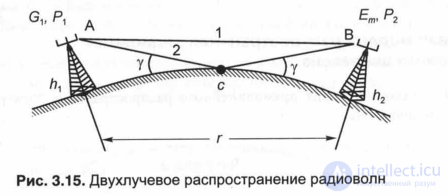
Fig. 3.15. Dual beam propagation

Thus, at the point of reception, there are only two beams that come into it with different amplitudes and phases. This is the idea of ​​the two-beam model of radio wave propagation. Depending on the ratio of the distance r and the line-of-sight distance r0 = 3.57 ([hi] 1/2 + [Li] 1/2), where hi and h2 are expressed in m, and r0 in km, the following formulas are possible to determine the strength fields at the receiving point, due to the interference of two rays:

a) in the general case, the amplitude value of the resulting electric field strength is determined by the formula (Fig. 3.15):

Et = 245 ^ PikbtG 'Ji + R2 + 2Rcos ( + - Ar), mV / m,

where R is the modulus of the reflection coefficient of electromagnetic waves of a given range from the earth; f is the phase loss angle at reflection; And g - the path difference of the rays: direct 1 and reflected 2 (Dg = [(AC + SV) - AB]), (Pi in kW, g in km, X and Dg in m).

Thus, compared with the single-beam model, the amplitude value of the electric field strength depends on the attenuation factor:

(3.75)

which, in turn, depends on the modulus of the reflection coefficient R, the phase loss angle φ upon reflection and the path difference of rays A. g. To determine R and φ, it is necessary to know the slip angle y, the type of polarization of the electromagnetic wave and the electrical constants (dielectric constant and electrical conductivity) reflective surface.

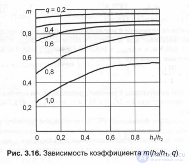
Approximate expression for A g is determined by the formula:

And g = Imhxh ^ r, (3.76)

where t is the coefficient depending on the ratio of the height of the receiving antenna (or reception point) above the ground h2 and the height of the transmitting antenna hi (for hi> h2), as well as the parameter

q = r / (2R-h1) ia, (3.77)

the coefficient mQi ^ hi, q) is determined from the graphs of fig. 3.16