Lecture
Consider the undirected graph G = ( V , E ).
An independent set of vertices (internally stable set) is a set of vertices of the graph G such that any two vertices in it are not adjacent, that is, no pair of vertices is connected by an edge. The set S ⊂ V satisfying the condition
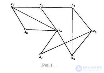
is called an independent set of vertices. For the graph shown in Figure 1, { x 7 , x 8 , x 2 }, { x 3 , x 1 } vertex sets are independent.
An independent set is called maximal when there is no other independent set into which it would belong. If the set satisfies condition (1) and condition
is a maximal independent set. For example, the sets { x 1 , x 3 , x 7 } and { x 4 , x 6 } are maximal independent, but { x 7 , x 8 , x 2 } are not. There can be more than one independent set in a graph.
If Q is a family of all independent sets of the graph G , then
is called the independence number of the graph G , and the set S * on which this maximum is reached is called the largest independent set.
There are n projects to be completed. To complete the project x i , a certain sub-volume R i of the available resources from the set {1, ..., p } is required. Let each project, given by a set of funds necessary for its implementation, can be executed in the same period of time. We construct a graph G , each vertex of which corresponds to a certain project, and an edge ( x i , x j ) to the availability of common means of support for projects x i and x j . The maximum independent set of the graph G represents the maximum set of projects that can be executed simultaneously in the same period of time.
In a dynamic system, there is a constant update of projects after a certain period of time, so that each time you need to repeat the procedure for building the maximum independent set in the corresponding graph G. In practice, it is not always possible to perform works corresponding to the maximum independent set. Then it is possible for each job (vertex x i ) to associate a certain penalty p i , which will increase with an increase in the time it takes to complete the job. At each moment in time, it is necessary to choose from the family of maximal independent sets such a set that maximizes a certain function of penalties on the vertices contained in the selected set.
The maximum complete subgraph (clique) of the graph G is a generated subgraph constructed on the subset S of the graph vertices and is complete and maximal in the sense that any other subgraph of the graph G constructed on the vertex set H containing S is not complete. That is, in contrast to the maximum independent set, in the click all the vertices are pairwise adjacent.
In the same way as the independence number of a graph was determined, using relation (3), we can determine the clique number of the graph (also known as density or density ). This is the maximum number of vertices in the clicks of this graph. Then, figuratively speaking, the “dense” graph will probably have a larger number, and the independence number will be smaller, while the “rarefied” graph will most likely have the opposite relationship between these numbers.
If the graph is small (for example, with the number of vertices not exceeding 20), then the maximum independent set can be constructed by sequential enumeration of independent sets with simultaneous testing of each set for maximalness. If there are many peaks, then this process becomes technically complex. The number of maximal independent sets increases, but during the search a large number of independent sets are formed, and then deleted, as it is found that they are contained in other previously obtained sets and therefore are not the maximum.
This algorithm is a significantly simplified search using a search tree. During the search, at some stage k , the independent set of vertices S k is expanded by adding to it a suitable selected vertex (to get a new independent set S k +1 ) at stage k +1, and this is done until the addition of vertices will become impossible, and the generated set will not become the maximum independent set. Let Q k be at the stage k the largest set of vertices for which S k ∩ Q k = Ø, that is, after adding any vertex from Q k to S k, we obtain an independent set S k +1 . At some arbitrary time of the algorithm, the Q k set consists of two types of vertices: Q k subsets — those vertices that were already used in the search process for extending S k sets, and Q k + subsets of such vertices that have not yet been used. Then further branching in the search tree includes the procedure for selecting the vertex x i k ∈ Q k + , adding it to S k to construct the set
and the generation of new sets:
and
The step of returning the algorithm is to remove the vertex x i k from S k +1 in order to return to S k , remove x i k from the old Q k + and add x i k to the old Q k - to form new Q k + and Q k - .
The set S k is a maximal independent set only when its further extension is impossible, that is, when Q k + = Ø. If Q k + ≠ Ø, then the current set S k was expanded at some previous stage of the algorithm by adding a vertex from Q k - , and therefore it is not a maximal independent set. Thus, a necessary and sufficient condition for the fact that S k is a maximum independent set is the fulfillment of equalities
If the next stage of the algorithm occurs when there exists a vertex x ∈ Q k - for which E ( x ) ∩ Q k + = Ø, then it doesn’t matter which of the vertices belonging to Q k + is used for the extension S k , and this is true for any number of further branches; the vertex x cannot be removed from Q p - at any next step p > k . Thus, the condition
is sufficient for the implementation of the return step, since with any further branching the maximum independent set cannot be obtained from S k .
As with any method using the search tree, it is advantageous here to strive to start the return steps as early as possible, since this will limit the “dimensions” of the “unnecessary” part of the search tree. Therefore, it is advisable to focus efforts on achieving condition (8) as soon as possible with the help of a suitable choice of vertices used in extending the sets S k . At each next step of the procedure, you can choose to add any vertex x i k ∈ Q k + to S k at the return stage x i k will be removed from Q k + and included in Q k - . If the vertex x k is chosen so that it belongs to the set E ( x ) for some vertex x from Q k - , then at the corresponding return step the value
decreases by one (in comparison with the value that was before the execution of the direct step in the return step), so condition (8) will now be fulfilled earlier.
Thus, one of the possible ways to select the vertex x i k to expand the set S k consists, first, in finding the vertex x * ∈ Q k - with the smallest possible value of Δ ( x * ) and, moreover, in choosing the vertex x i from the set E ( x * ) ∩ Q k + . Such a choice of the vertex x i k will result in a return step to a decrease in the value of Δ ( x * ) - each time by one - until the vertex x * satisfies condition (8) when performing the return step.
It should be noted that since at the return step, the vertex x i k falls into Q k - , it may turn out that with this new input the value of Δ is less than for the previously fixed vertex x * . Therefore, it is necessary to check whether this new vertex will accelerate the fulfillment of condition (8). This is especially important at the beginning of branching, when Q k - = Ø.
For the graph G = ( V , E ), the dominant set of vertices (also called the externally stable set ) is the set of vertices S ⊆ E chosen so that for every vertex x j that is not in S , there is an arc coming from some vertex of S at the vertex x j .
Thus, S is the dominant set of vertices if
For the graph shown in Fig. 2, the vertex sets { x 1 , x 4 , x 6 }, { x 1 , x 4 }, { x 3 , x 5 , x 6 } are the dominant sets.
A dominant set is said to be minimal if there is no other dominant set contained in it.
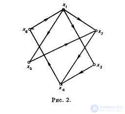
A set S is a minimal dominant set if it satisfies relation (10) and there is no proper subset in S that satisfies a condition similar to (10). So, for example, for the graph shown in fig. 2, the set { x 1 , x 4 } is minimal, but { x 1 , x 4 , x 6 } is not. The minimum dominant set is also the set { x 3 , x 5 , x 6 }, and there are still several such sets in this graph. Consequently, as in the case of maximal independent sets, there can be several minimal dominant sets in the graph, and they do not necessarily contain the same number of vertices.
If P is a family of all minimal dominant sets of a graph, then the number
is called the domination number of the graph G , and the set S * on which the minimum is reached is called the smallest dominant set.
For the graph shown in Fig. 2, the smallest dominant set is the set { x 1 , x 4 } and, therefore, β [ G ] = 2.
Let A t be the transposed adjacency matrix of a graph G with unit diagonal elements. The task of determining the smallest dominant set of a graph G is equivalent to the problem of finding such a smallest set of columns in the matrix A t such that each row of the matrix contains one in at least one of the selected columns. This last task of finding the smallest set of columns “covering” all the rows was studied quite intensively under the name of the least coverage problem (GCP).
In a common RFP, a matrix consisting of 0 and 1 is not necessarily square. In addition, each column j (in our case, each vertex x j ) is assigned a certain cost c j and it is required to choose a covering (or, in another terminology, for the case of graphs, the dominant set of vertices) with the lowest total cost). Since the task of constructing the smallest dominant set of vertices is a very special problem of coverage with c j = 1 for all j = 1, ..., n , at first glance it seems that finding such a set is actually much easier than solving a general RFP.
The RFP is obliged by its name to the following set-theoretic interpretation. Given the set R = { r 1 , ..., r M } and the family I = { S 1 , ..., S N } of the sets S j ⊂ R. Any subfamily I ′ = { S j 1 , S j 2 , ..., S j k } of the family I , such that
is called a covering of the set R , and the sets S j i are called covering sets . If, together with relation (12), I ′ satisfies the condition
that is, the sets S j i { i = 1, ..., k } do not overlap in pairs, it is called a partition of the set R.
If each S j ∈ I is associated with a positive cost c j , then the RFP is formulated as follows: find the covering of the set R , which has the lowest cost, and the cost of the family I ′ = { S j 1 , ..., S j k } is defined as ∑ i = 1 k c j i . The problem of the smallest partitioning (ZNR) is also formulated in the same way.
Due to the special nature of the RFP, it is often possible to draw certain well-known conclusions and simplifications in its study. For example:
Suppose that all these simplifications are made (if they are possible) and that the original RFP is already reformulated in the corresponding irreducible form.
ZNR is closely related to the RFP, being essentially an RFP with an additional restriction (non-overlap). This restriction is beneficial if the problem is solved with the help of some method using the search tree: with such restrictions it may be found out early that some possible tree branches should not be considered,
Simple methods for solving SNR using the search tree were proposed by Pierce, Garfinkel and Nemhauzero.
The essence of these methods is as follows. First, “blocks” of columns are built, one for each element r k of R , that is, there are a total of M blocks, the k -th block consists of such sets of family I (represented by columns) that contain the element r i but no elements with smaller indices - r 1 , ..., r k −1 . Therefore, each set (column) appears in exactly one particular block and the set of blocks can be represented as a table. In specific tasks, some of the blocks may be missing.
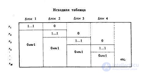
In the process of the algorithm, the blocks are searched sequentially and the formation of the k-th block begins after each element, r i 1 ≤ i ≤ k - 1, is covered by a particular solution. Thus, if some set in block k contains elements with indices less than k , then it must be dropped (at this stage) in accordance with the requirement of non-overlap. Sets within each block are placed in ascending order of their costs and renumbered so that S k now stands for the set corresponding to the jth column of the table.
The current “best” solution B ′ with the cost z ′ is known at any stage of the search ( B ′ denotes the family of the corresponding covering sets). If B and z are the corresponding family and cost at this stage of the search, and E is a set representing those elements (i.e., strings) r i that are covered by sets from B , then one of the simple algorithms using the search tree can be entered in the following way.
If the search ends with the exhaustion of block 1 (see step 4), then it is advisable to rearrange the blocks in ascending order of the number of columns (sets) in each block. This can be done (before building the source table) by renumbering the elements (rows) r 1 ... r M in order of increasing the number of sets from S containing the corresponding elements.
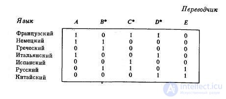
Suppose that an organization needs to hire French, German, Greek, Italian, Spanish, Russian, and Chinese translators into English and that there are five candidates A , B , C , D, and E. Each candidate owns only a certain subset of the above set of languages and requires a well-defined salary. It is necessary to decide which translators (from the above languages to English) should be hired so that the cost of the salary is the lowest. This is the least coverage problem.
Если, например, требования на оплату труда у всех претендентов одинаковые и группы языков, на которых они говорят, указаны ниже в матрице Т, то решение задачи будет таким: нужно нанять переводчиков В , С , D .
Предположим, что некоторое количество единиц информации хранится в N массивах длины c j , j = 1, 2, …, N , причем на каждую единицу информации отводится по меньшей мере один массив. В некоторый момент делается запрос о М единицах информации. Они могут быть получены различными способами при помощи поиска в массиве. Для того чтобы получить все M единиц информации и при этом произвести просмотр массивов наименьшей длины, надо решить ЗНП, вкоторой элемент t i j матрицы T равен 1, если информация i находится в массиве, и 0 в противном случае.
Пусть вершины неориентированного графе G представляют аэропорты, а дуги графа G — этапы полетов (беспосадочные перелеты), которые осуществляются в заданное время. Любой маршрут в этом графе (удовлетворяющий ряду условий, которые могут встретиться на практике) соответствует некоторому реально выполнимому маршруту полета. Пусть имеется N таких возможных маршрутов и для каждого из них каким-то способом подсчитана его стоимость (например, стоимость j -го маршрута равна c j ). Задача нахождения множества маршрутов, имеющего наименьшую суммарную стоимость и такого, что каждый этап полета содержится хотя бы в одном выбранном маршруте, является задачей о наименьшем покрытии с матрицей Т= [ t ij ] in which the element t ij is equal to 1 if the i- th stage is contained in the j- th route, and is equal to 0 otherwise.

Comments
To leave a comment
Algorithms
Terms: Algorithms