Lecture
All algorithms considered in the previous sections have one fatal flaw - the time of their execution is of the order of n 2 . This makes sorting large amounts of data very slow. In essence, at some point, these algorithms become too slow to use them [1] . Unfortunately, the scary stories about "sorting that lasted three days," are often real. When sorting takes too much time, the reason for this is usually the inefficiency of the algorithm used in it. However, the first reaction in such a situation often becomes manual code optimization, possibly by rewriting it in an assembler. Despite the fact that manual optimization sometimes speeds up the procedure by a constant factor [2] , if the sorting algorithm is not efficient, the sorting will always be slow no matter how optimally the code is written. It should be remembered that if the time of the procedure is proportional to n 2 , then an increase in the speed of the code or computer will give only a slight improvement [3] , since the execution time increases as n 2 . (Actually, curve n 2 in Fig. 21.1 (bubble sort) is stretched to the right, but otherwise corresponds to reality.) There is a rule: if the algorithm used in the program is too slow by itself, no amount of manual optimization will make the program fast enough. The solution is to use a better sorting algorithm.
The following are two excellent sorting methods. The first is called Shell sorting . The second - quick sorting - is usually considered the best sorting algorithm. Both methods are more advanced sorting methods and have much better overall performance than any of the simple methods above.
Shell sorting is so named after its author, Donald L. Shell (Donald Lewis Shell) [4] . However, this name was fixed, probably also because the effect of this method is often illustrated by rows of sea shells overlapping each other (in English "shell" - "shell"). The general idea is borrowed from sorting inserts and is based on reducing steps [5] . Consider the diagram in fig. 21.2. First, all the elements that are separated by three positions are sorted. Then sorted elements located at a distance of two positions. Finally, all neighboring elements are sorted.
Fig. 21.2. Shell sort Pass 1 fdacbe
\ ___ \ ___ \ ___ / / /
\ ___ \ _____ / /
\ _______ /
Pass 2 cbafde
\ ___ \ ___ | ___ | ___ / /
\ ______ | ______ /
Pass 3 abcdef
| ___ | ___ | ___ | ___ | ___ |
Abcdef result
|
The fact that this method gives good results, or even the fact that it sorts an array in general, is not so easy to see. However, this is true. Each pass of sorting extends to a relatively small number of elements or to elements that are already in a relative order. Therefore, Shell sorting is effective, and each pass increases orderliness [6] .
The specific sequence of steps may be different. The only rule is that the last step be 1. For example, the following sequence:
9, 5, 3, 2, 1
gives good results and is used in the Shell sorting implementation shown here. Sequences that are powers of 2 should be avoided - for mathematically complex reasons, they reduce the sorting efficiency (but the sorting still works!).
  / * Shell sort.  * /
 void shell (char * items, int count)
 {

   register int i, j, gap, k;
   char x, a [5];

   a [0] = 9;  a [1] = 5;  a [2] = 3;  a [3] = 2;  a [4] = 1;

   for (k = 0; k <5; k ++) {
     gap = a [k];
     for (i = gap; i <count; ++ i) {
       x = items [i];
       for (j = i-gap; (x <items [j]) && (j> = 0); j = j-gap)
         items [j + gap] = items [j];
       items [j + gap] = x;
     }
   }
 }
You may have noticed that the inner for loop has two check conditions. Obviously, comparing x <items [j] is necessary for the sorting process. The expression j> = 0 prevents the items array from escaping . These additional checks somewhat reduce the sorting performance of Shell.
In slightly modified versions of this sorting method, special elements of the array are used, called signal labels . They do not belong to the actually sorted array, but contain special values corresponding to the smallest possible and largest possible elements [7] . This eliminates the need to check the output of the array. However, the use of signal labels of elements requires specific information about the data being sorted, which reduces the universality of the sorting function.
Shell sorting analysis is associated with very complex mathematical problems that go far beyond the scope of this book. Take for granted that the sorting time is proportional
n 1,2
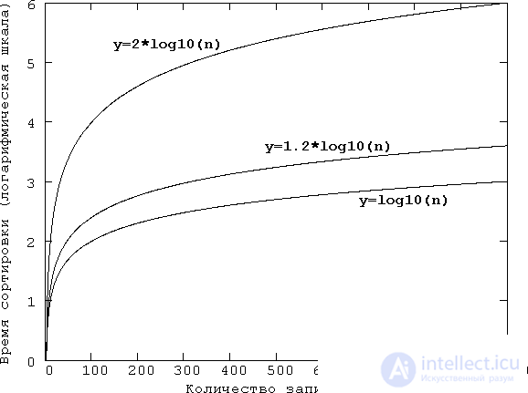
when sorting n elements [8] . And this is already a significant improvement compared with sortings of order n 2 . To understand how big it is, refer to fig. 21.3, which shows the graphs of the functions n 2 and n 1,2 . However, one should not overly admire Shell sorting - quick sorting is even better.
Fig. 21.3. Attempt to visualize the curves n 2 and n 1,2 . Although it is not possible to draw these curves with exact observance of the scale for changing the number of records (n), for example, in the interval from 0 to 1000, for example, it is possible to get an idea of the behavior of these curves using the graphs of the functions y = (n / 100) 2 and y = (n / 100) 1,2 . For comparison, we also plotted a straight line y = n / 100. In addition, in order to get an idea of the growth of these curves, one can take a logarithmic scale on the ordinate axis — it’s like drawing the logarithms of these functions.
Quick sorting, invented by Charles A. R. Hoare [9] (Charles Antony Richard Hoare) and named after him, is the best sorting method presented in this book and is generally considered the best general-purpose sorting algorithm currently available. It is based on sorting exchanges - an amazing fact, given the terrible performance of bubble sorting!
Quick sort is based on the idea of division. The general procedure is to select a value, called the comparand [10] , and then split the array into two parts. All elements larger or equal to the comparand are moved to one side and smaller to the other. Then this process is repeated for each part until the array is sorted. For example, if the source array consists of fedacb characters, and the d symbol is used as a comparant, the first pass of the quick sort will rearrange the array as follows:
  Start fedacb

 Pass 1 bcadef
Then the sorting is repeated for both halves of the array, i.e. bca and def . As you can see, this process is inherently recursive, and, indeed, in its pure form, quick sorting is implemented as a recursive function [11] .
The value of the comparand can be selected in two ways - randomly or by averaging a small number of values from the array. For optimal sorting, you must choose a value that is located exactly in the middle of the range of all values. However, for most data sets this is not easy. In the worst case, the selected value is one of the last. However, even in this case, the quick sort works correctly. In the quick sort version below, the middle element of the array is selected as the comparand.
  / * Function, quick sort function.  * /
 void quick (char * items, int count)
 {
   qs (items, 0, count-1);
 }

 / * Quick sort.  * /
 void qs (char * items, int left, int right)
 {
   register int i, j;
   char x, y;

   i = left;  j = right;
   x = items [(left + right) / 2];  / * selection of the frame * /

   do {
     while ((items [i] <x) && (i <right)) i ++;
     while ((x <items [j]) && (j> left)) j--;

     if (i <= j) {
       y = items [i];
       items [i] = items [j];
       items [j] = y;
       i ++;  j--;
     }
   } while (i <= j);

   if (left <j) qs (items, left, j);
   if (i <right) qs (items, i, right);
 }
In this version, the quick () function prepares a call to the qs () main sorting function. This provides a common interface with the items and count parameters, but not essential, since you can call the qs () function directly with three arguments.
Obtaining the number of comparisons and exchanges that are performed during quick sorting requires mathematical calculations that are beyond the scope of this book. However, the average number of comparisons is
n log n
and the average number of exchanges is approximately equal to
n / 6 log n
These values are much smaller than the corresponding characteristics of the sorting algorithms considered earlier.
It is worth mentioning one particularly problematic aspect of quick sorting. If the value of the comparand in each division is equal to the largest value, the quick sort becomes a “slow sort” with a runtime of the order of n 2 . Therefore, carefully choose the method of determining the Comparand. This method is often determined by the nature of the data being sorted. For example, in very large mailing lists, in which sorting occurs by zip code, the choice is simple, because zip codes are fairly evenly distributed — the comparade can be determined using a simple algebraic function. However, in other databases, a random value is often the best choice. A popular and fairly effective method is to select three elements from the sorting part of the array and take the value between the other two as a comparand.

[1] Of course, this does not mean that the function f (n) = n 2 at some point increases in steps. Not at all! Simply by increasing the size of the array n, the sorting character changes; from the internal, it actually becomes external , when the array does not fit in the RAM and intensive page paging begins, and after it the virtual memory mechanism slips. These events may indeed come suddenly, and then it may seem that a slight increase in the sorted array or simply adding some absolutely insignificant task will lead to a catastrophic increase in the sorting time (for example, dozens of times!).
[2] Individual programmers - "lovers of stories about fishing" - swear about the increase in efficiency, first half, then twice or three times, by the middle of the story - an order of magnitude, and by the end of the story - several orders of magnitude. (This does not work out even in specially selected examples for an advertising brochure on the Assembly language.) In fact, the performance may even fall. In the best case, it is possible to increase it by 10-12% for really significant production tasks. In this case, the more complex the algorithm, the more difficult it is to rewrite it in Assembler and the easier it is to make a mistake in it during rewriting, and the more difficult it is to find it. In addition, this factor should be taken into account: for example, a programmer wrote a programmer who chose a simple (but not very effective - what he knew about) algorithm because managers insisted that the program be completed as soon as possible, and the same managers will be assigned to not very qualified specialists! The effect will indeed be several orders of magnitude greater, but in a completely opposite direction! After all, with the same success for the "improvement" of Shakespeare's tragedies for typewriters it was possible to seat a herd of monkeys!
[3] Indeed, in order to increase the size of the array being sorted by m times while preserving the sorting time, the processor speed will have to be increased m 2 times, provided that the access time to the array elements does not increase, i.e. For example, the efficiency of paging will not decrease.
[4] It is believed that Donald L. Shell described his sorting method on July 28, 1959. This method is classified as merge with exchange ; often referred to as descending sorting .
[5] Step - the distance between the sorted items at a particular sorting stage.
[6] That is, reduces the number of disturbances (inversions).
[7] -∞ and + ∞.
[8] Generally speaking, Shell's sorting time depends on the sequence of steps. (However, the minimum is, of course, n log 2 n .) The optimal sequence is not known until now. Donald Knut researched various sequences (without forgetting the Fibonacci sequence). In fact, he concluded that there was some sort of “witchcraft” in determining the best sequence. In 1969, Vogan Pratt discovered that if all the steps are chosen from a set of numbers of the form 2 p 3 q less than n, then the running time will be of the order of n (log n) 2 . A.A. Papernov and G.V. In 1965, Stasevich proved that the maximum Shell sorting time does not exceed O (n 1.5 ), and it is impossible to reduce the rate by 1.5. A large number of experiments with Shell sorting were conducted by James Peterson and David L. Russell at Stanford University in 1971. They tried to determine the average number of displacements at 100≤ n ≤250`000 for a sequence of steps 2 k -1. The most appropriate formulas were 1.21 n 1.26 and, 39 n (ln n ) -2.33 n ln n . But when the range n is changed, it turned out that the coefficients in the representation by a power function practically do not change, and the coefficients in the logarithmic representation change quite dramatically. Therefore, it is natural to assume that it is the power function that describes the true asymptotic behavior of the Shell sort.
[9] There is also the writing of C. Э. R. Hoor.
[10] Comparand - operand in the comparison operation. Sometimes referred to as the basis and criterion of the partition
[11] If you want to avoid recursion, do not worry, everything is very easy to rewrite even for Fortran IV, you can easily find the necessary non-recursive option in the previously mentioned literature.

Comments
To leave a comment
Algorithms
Terms: Algorithms