Lecture
One of the methods of systematically traversing the vertices of a graph is called depth-first search . The depth-first search strategy, as its name implies, is to go "in depth" of the graph as far as possible. When performing a depth search, all edges that go out of a vertex opened by the last one are examined and leave the top only when no unexplored edges remain - this returns to the top from which the top v was opened. This process continues until all the vertices reachable from the original are opened. If at the same time there are undiscovered vertices, then one of them is selected as the new original vertex and the search is repeated from it. This process is repeated until all vertices are open.
When vertex v is opened in the process of scanning the adjacency list of an already open vertex, the search procedure records this event by setting the predecessor's field v prev [v] to u. Unlike the search in width, where the preceding subgraph forms a tree, when searching in depth, the preceding subgraph can consist of several trees , since the search can be performed from several original vertices.
As in the process of performing the search in width, the vertices of the graph are colored in different colors indicating their condition. Each vertex is initially white, then when it opens (discover), it turns gray in the search process, and when it finishes (finish), when its adjacency list is completely scanned, it turns black. This technique ensures that each vertex is ultimately located in only one depth-first search tree.
In addition to building a search depth forest, depth search also places timestamps on vertices. Each vertex has two such labels — the first d [v] , which indicates when the vertex y opens (and turns gray), and the second — f [v] , which captures the moment when the search completes scanning the adjacency list of j and she turns black. These tags are used by many algorithms and are useful when considering the depth of search behavior.
  DFS (G)
 1 for (For) each vertex u є V [G)
 2 do color [u] "- WHITE
 3 prev [u] "- NIL
 4 time "- About
 5 for (For) each vertex u E V [G]
 6 do if color [u] = white
 7 then DFS_Visit (u)

 DFS_Visit (u)
 1 color [u] "- GRAY // White top open u
 2 time "- time + 1
 3 d [u] «- time
 4 for (For) each vertex v є Adj [u] // Investigation of the edge (u, v).
 5 do if color [v] = white
 6 then prev [v] "- u
 1 DFS_Visit (v)
 8 color [u] "- BLACK // End
 9 f [u] "- time " - time +1
In lines 1-3, all vertices are painted white, and their fields nx are initialized to nil. Line 4 resets the global time counter. In lines 5-7, all vertices from V are checked alternately, and when a white vertex is detected, it is processed using the DFS_Visit procedure. Each time you call the DFS_Visit (u) procedure on line 7, the vertex becomes the root of the new tree in the search for depth forest. When returning from the DFS procedure, each vertex is matched with two points in time — the discovery time d [u] and the finishing time (f time) f [u].
Each time DFS_Visit (ix) is called, the vertex is initially white. In line 1 it is colored gray, in line 2 the global variable time increases, and in line 3 the new value of the variable time is recorded in the open time field d [u] . In lines 4-7, all vertices adjacent to u are examined, and recursive visits to white vertices are performed. When considering row 4 vertices v є Adj [and], we say that the edge ( u, v ) is explored by depth-first search. Finally, after all edges leaving u are examined, lines 8–9 are vertex and colored black, and the time for completing work with it is recorded in the f [u] field.
Cycles in lines 1-3 and 5-7 of the DFS procedure are performed in the o (V) time, excluding the time required to call the DFS_Visit procedure. The DFS_VISIT procedure is called exactly once for each vertex v є V, since it is called only for white vertices, and the first thing it does is to color the vertex passed as a parameter to gray. During the execution of DFS_Visit (v), the loop in lines 4-7 is executed | Adj [v] | time. Insofar as
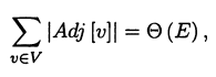
The total cost of executing lines 4-7 of the DFS_Visit procedure is o (E).
The running time of the DFS procedure is thus o (V + E) .
Depth traversal order: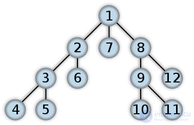
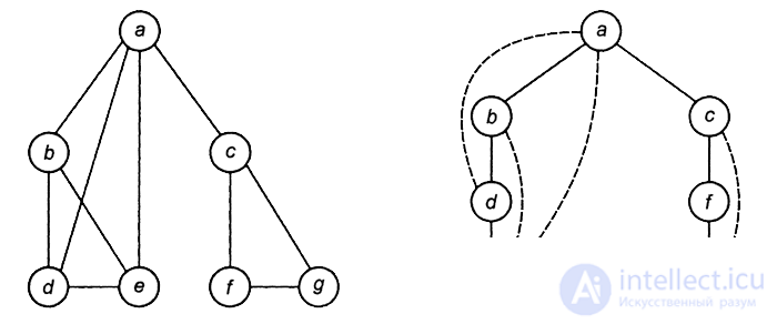
The graph and spanning tree obtained by traversing its vertices using the depth search method:
Search in depth (English depth-first search, DFS) is a recursive algorithm for traversing graph vertices. If the search method in width was made symmetrically (the vertices of the graph were viewed through the levels), then this method assumes progress inwards as long as possible. The impossibility of further advancement means that the next step will be a transition to the last one, which has several movement variants (one of which has been studied completely), a previously visited node (vertex). The absence of the latter indicates one of two possible situations: either all the vertices of the graph have already been viewed, or all those that are accessible from the vertex taken as the initial one, but not all (disconnected and oriented graphs allow the last option).
Consider how the algorithm will behave using a specific example. The following undirected connected graph has 5 vertices in total. 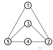 First you need to select the starting vertex. Whatever vertex is chosen as such, the graph is completely investigated anyway, since, as already mentioned, this is a connected graph without a single directed edge.
Let the tour begin at node 1, then the order of the sequence of scanned nodes will be as follows: 1 2 3 5 4. If you start the execution, for example, from node 3, then the order of the walk will be different: 3 2 1 5 4.
The depth-first search algorithm is based on recursion, i.e., the bypass function, as it executes, calls itself, which makes the code as a whole rather compact. Pseudocode algorithm:
DFS (st) function header
Print (st)
visited [st] ← visited;
For r = 1 to n perform
If (graph [st, r] ≠ 0) and (visited [r] not visited) then DFS (r)
Here DFS (depth-firstsearch) is the name of the function. Its only parameter st is the starting node, which is passed from the main part of the program as an argument. Each of the elements of the visited logical array is preset to false, that is, each of the vertices will initially be listed as not visited. A two-dimensional graph array is a graph adjacency matrix. Most of the attention should be concentrated on the last line. If an element of the adjacency matrix, at some step, is 1 (and not 0) and the vertex with the same number as the checked column of the matrix was not visited, the function recursively repeats. Otherwise, the function returns to the previous recursion stage.
| one 2 3 four five 6 7 eight 9 ten eleven 12 13 14 15 sixteen 17 18 nineteen 20 21 22 23 24 25 26 27 28 29 thirty 31 32 33 34 35 36 37 38 39 40 41 42 43 44 45 46 |
#include "stdafx.h"
#include using namespace std; const int n = 5; int i, j; bool * visited = new bool [n]; // graph adjacency matrix int graph [n] [n] = { {0, 1, 0, 0, 1}, {1, 0, 1, 1, 0}, {0, 1, 0, 0, 1}, {0, 1, 0, 0, 1}, {1, 0, 1, 1, 0} }; // search in depth void DFS (int st) { int r; cout << st + 1 << ""; visited [st] = true; for (r = 0; r <= n; r ++) if ((graph [st] [r]! = 0) && (! visited [r])) DFS (r); } // main function void main () { setlocale (LC_ALL, "Rus"); int start; cout << "Graph adjacency matrix:" << endl; for (i = 0; i { visited [i] = false; for (j = 0; j cout << "" << graph [i] [j]; cout << endl; } cout << "Starting Top >>"; cin >> start; // array of visited vertices bool * vis = new bool [n]; cout << "Bypass order:"; DFS (start-1); delete [] visited; system ("pause >> void"); } |
| one 2 3 four five 6 7 eight 9 ten eleven 12 13 14 15 sixteen 17 18 nineteen 20 21 22 23 24 25 26 27 28 29 thirty 31 32 33 34 35 36 37 |
program DepthFirstSearch;
uses crt; const n = 5; var i, j, start: integer; visited: array [1..n] of boolean; const graph: array [1..n, 1..n] of byte = ((0, 1, 0, 0, 1), (1, 0, 1, 1, 0), (0, 1, 0, 0, 1), (0, 1, 0, 0, 1), (1, 0, 1, 1, 0)); {depth search} procedure DFS (st: integer); var r: integer; begin write (st: 2); visited [st]: = true; for r: = 1 to n do if (graph [st, r] <> 0) and (not visited [r]) then DFS (r); end; {main program block} begin clrscr; writeln ('Adjacency matrix:'); for i: = 1 to n do begin visited [i]: = false; for j: = 1 to n do write (graph [i, j], ''); writeln; end; write ('Starting vertex >>'); read (start); writeln ('Traversal Result'); DFS (start); end. |
For ease of understanding the result of two programs, taken undirected graph, given earlier as an example, and represented by the adjacency matrix graph [5] [5].

Comments
To leave a comment
Algorithms
Terms: Algorithms