Lecture
The Little algorithm is used to find solutions to the traveling salesman problem in the form of a Hamiltonian contour . This algorithm is used to find the optimal Hamiltonian contour in a graph with N vertices, each vertex i being connected to any other vertex j by a bidirectional arc. Each arc is assigned a weight Сi, j, and the weights of the arcs are strictly positive (Сi, j ≥ 0). The weights of the arcs form a cost matrix. All elements along the diagonal of the matrix equate to infinity (Cj, j = ∞).
If the pair of vertices i and j is not interconnected (the graph is not fully connected), then we assign to the corresponding element of the cost matrix a weight equal to the length of the minimum path between the vertices i and j. If in the end the arc (i, j) enters the resulting contour, then it must be replaced by the corresponding path. The matrix of optimal paths between all vertices of the graph can be obtained by applying the Danzig or Floyd algorithm.
The Little’s algorithm is a special case of applying the branch and bound method to a specific problem. The general idea is trivial: you need to divide a huge number of enumerated variants into classes and get estimates (from below - in the minimization problem, from above - in the maximization problem) for these classes, in order to be able to discard the variants not by one, but by whole classes. The difficulty is to find such a division into classes (branches) and such assessments (boundaries) so that the procedure is effective.
Little algorithm
During the solution, the current value of the lower limit is continuously calculated. The lower bound is the sum of all subtracted items in the rows and columns. The final value of the lower bound should coincide with the length of the resulting contour.
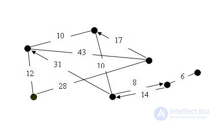
It is necessary to find the best route for a traveling salesman in the graph presented in the figure:
Let us number the vertices of the original graph, and compose a matrix of lengths of shortest arcs between each pair of vertices D0, if there is no arc between the vertex i and j, the value ∞ is assigned to the matrix element di, j. The original graph with numbered vertices is shown in the figure below.
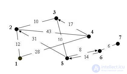
Matrix D0:
| D0 = | 0 | 12 | ∞ | 28 | ∞ | ∞ | ∞ |
| 12 | 0 | ten | 43 | ∞ | ∞ | ∞ | |
| ∞ | ten | 0 | ∞ | ten | ∞ | ∞ | |
| 28 | 43 | 17 | 0 | ∞ | ∞ | ∞ | |
| ∞ | 31 | ten | ∞ | 0 | eight | ∞ | |
| ∞ | ∞ | ∞ | ∞ | 14 | 0 | 6 | |
| ∞ | ∞ | ∞ | ∞ | ∞ | 6 | 0 |
The matrix D0 contains elements with values of ∞, which is not permissible. Replace the infinite arcs by the length of the shortest paths between the corresponding vertices (with the exception of the diagonal elements to which we assign infinity values). As a result, we obtain the following cost matrix:
| ∞ | 12 | 22 | 28 | 32 | 40 | 46 |
| 12 | ∞ | ten | 40 | 20 | 28 | 34 |
| 22 | ten | ∞ | 50 | ten | 18 | 24 |
| 28 | 27 | 17 | ∞ | 27 | 35 | 41 |
| 32 | 20 | ten | 60 | ∞ | eight | 14 |
| 46 | 34 | 24 | 74 | 14 | ∞ | 6 |
| 52 | 40 | thirty | 80 | 20 | 6 | ∞ |
Since its elements are no longer arcs but distances between vertices, we are freed from the need to check the triangle inequality (in this case, it is performed automatically).
We will find the minimum elements in each line and then subtract it from the remaining elements of the line (the minimum elements are written opposite the corresponding lines). We get the matrix presented below.
| one | 2 | 3 | four | five | 6 | 7 | |
| one | ∞ | 0 | ten | sixteen | 20 | 28 | 34 |
| 2 | 2 | ∞ | 0 | thirty | ten | 18 | 24 |
| 3 | 12 | 0 | ∞ | 40 | 0 | eight | 14 |
| four | eleven | ten | 0 | ∞ | ten | 18 | 24 |
| five | 24 | 12 | 2 | 52 | ∞ | 0 | 6 |
| 6 | 40 | 28 | 18 | 68 | eight | ∞ | 0 |
| 7 | 46 | 34 | 24 | 74 | 14 | 0 | ∞ |
We will do the same for non-zero columns. We obtain a matrix containing zeros in each row and each column.
| one | 2 | 3 | four | five | 6 | 7 | |
| one | ∞ | 0 | ten | 0 | 20 | 28 | 34 |
| 2 | 0 | ∞ | 0 | 14 | ten | 18 | 24 |
| 3 | ten | 0 | ∞ | 24 | 0 | eight | 14 |
| four | 9 | ten | 0 | ∞ | ten | 18 | 24 |
| five | 22 | 12 | 2 | 36 | ∞ | 0 | 6 |
| 6 | 38 | 28 | 18 | 52 | eight | ∞ | 0 |
| 7 | 44 | 34 | 24 | 58 | 14 | 0 | ∞ |
For each zero element, we calculate the value Гij equal to the sum of the smallest element i of the row (excluding the element Сij = 0) and the smallest element j of the column.
G1,2 = 0, G1.4 = 14, G2.1 = 9, G2.3 = 0, G3.2 = 0, G3.5 = 8, G4.3 = 9, G5.6 = 2, G6, 7 = 14, G7.6 = 14,
As a result of the comparison, we obtained 3 identical maximal G = 14. This means that the algorithm forks and we must consider all the resulting options one by one. Consider option G1.4 = 14
We remove from the cost matrix row 1 and column 4. We enter an arc (1,4) into the current oriented graph
| one | 2 | 3 | five | 6 | 7 | |
| 2 | 0 | ∞ | 0 | ten | 18 | 24 |
| 3 | ten | 0 | ∞ | 0 | eight | 14 |
| four | 9 | ten | 0 | ten | 18 | 24 |
| five | 22 | 12 | 2 | ∞ | 0 | 6 |
| 6 | 38 | 28 | 18 | eight | ∞ | 0 |
| 7 | 44 | 34 | 24 | 14 | 0 | ∞ |
In line 4 and column 1 there is no element equal to ∞. Assign the infinity value to the element (4.1) to avoid premature loop closure.
Current Lower Bound = 87
The lower bound is the sum of all subtracted items in the rows and columns. The final value of the lower bound should coincide with the length of the resulting contour.
We will find the minimum elements in each line and then subtract it from the remaining elements of the line (the minimum elements are written opposite the corresponding lines). We get the matrix presented below.
| one | 2 | 3 | five | 6 | 7 | |
| 2 | 0 | ∞ | 0 | ten | 18 | 24 |
| 3 | ten | 0 | ∞ | 0 | eight | 14 |
| four | ∞ | ten | 0 | ten | 18 | 24 |
| five | 22 | 12 | 2 | ∞ | 0 | 6 |
| 6 | 38 | 28 | 18 | eight | ∞ | 0 |
| 7 | 44 | 34 | 24 | 14 | 0 | ∞ |
We will do the same for non-zero columns. We obtain a matrix containing zeros in each row and each column.
| one | 2 | 3 | five | 6 | 7 | |
| 2 | 0 | ∞ | 0 | ten | 18 | 24 |
| 3 | ten | 0 | ∞ | 0 | eight | 14 |
| four | ∞ | ten | 0 | ten | 18 | 24 |
| five | 22 | 12 | 2 | ∞ | 0 | 6 |
| 6 | 38 | 28 | 18 | eight | ∞ | 0 |
| 7 | 44 | 34 | 24 | 14 | 0 | ∞ |
For each zero element, we calculate the value Гij equal to the sum of the smallest element i of the row (excluding the element Сij = 0) and the smallest element j of the column.
G2,1 = 10, G2.3 = 0, G3.2 = 10, G3.5 = 8, G4.3 = 10, G5.6 = 2, G6.7 = 14, G7.6 = 14,
As a result of the comparison, we obtained 2 identical maximal G = 14. This means that the algorithm forks and we must consider all the resulting options one by one. Consider option G6.7 = 14
Remove from the cost matrix row 6 and column 7. We enter in the current oriented graph an arc (6.7)
| one | 2 | 3 | five | 6 | |
| 2 | 0 | ∞ | 0 | ten | 18 |
| 3 | ten | 0 | ∞ | 0 | eight |
| four | ∞ | ten | 0 | ten | 18 |
| five | 22 | 12 | 2 | ∞ | 0 |
| 7 | 44 | 34 | 24 | 14 | 0 |
In line 7 and column 6 there is no element equal to ∞. Assign the infinity value to the element (7,6) to avoid premature loop closure.
Current Lower Bound = 87
We will find the minimum elements in each line and then subtract it from the remaining elements of the line (the minimum elements are written opposite the corresponding lines). We get the matrix presented below.
| one | 2 | 3 | five | 6 | |
| 2 | 0 | ∞ | 0 | ten | 18 |
| 3 | ten | 0 | ∞ | 0 | eight |
| four | ∞ | ten | 0 | ten | 18 |
| five | 22 | 12 | 2 | ∞ | 0 |
| 7 | thirty | 20 | ten | 0 | ∞ |
We will do the same for non-zero columns. We obtain a matrix containing zeros in each row and each column.
| one | 2 | 3 | five | 6 | |
| 2 | 0 | ∞ | 0 | ten | 18 |
| 3 | ten | 0 | ∞ | 0 | eight |
| four | ∞ | ten | 0 | ten | 18 |
| five | 22 | 12 | 2 | ∞ | 0 |
| 7 | thirty | 20 | ten | 0 | ∞ |
For each zero element, we calculate the value Гij equal to the sum of the smallest element i of the row (excluding the element Сij = 0) and the smallest element j of the column.
G2,1 = 10, G2.3 = 0, G3.2 = 10, G3.5 = 0, G4.3 = 10, G5.6 = 10, G7.5 = 10,
As a result of the comparison, we obtained 5 identical maximal G = 10. This means that the algorithm forks and we must consider all the resulting options one by one. Consider the option G2.1 = 10
Remove from the cost matrix row 2 and column 1. We enter in the current oriented graph an arc (2.1)
| 2 | 3 | five | 6 | |
| 3 | 0 | ∞ | 0 | eight |
| four | ten | 0 | ten | 18 |
| five | 12 | 2 | ∞ | 0 |
| 7 | 20 | ten | 0 | ∞ |
In line 4 and column 2 there is no element equal to ∞. Assign the infinity value to the element (4.2) to avoid premature loop closure.
Current Lower Bound = 101
We will find the minimum elements in each line and then subtract it from the remaining elements of the line (the minimum elements are written opposite the corresponding lines). We get the matrix presented below.
| 2 | 3 | five | 6 | |
| 3 | 0 | ∞ | 0 | eight |
| four | ∞ | 0 | ten | 18 |
| five | 12 | 2 | ∞ | 0 |
| 7 | 20 | ten | 0 | ∞ |
We will do the same for non-zero columns. We obtain a matrix containing zeros in each row and each column.
| 2 | 3 | five | 6 | |
| 3 | 0 | ∞ | 0 | eight |
| four | ∞ | 0 | ten | 18 |
| five | 12 | 2 | ∞ | 0 |
| 7 | 20 | ten | 0 | ∞ |
For each zero element, we calculate the value Гij equal to the sum of the smallest element i of the row (excluding the element Сij = 0) and the smallest element j of the column.
G3,2 = 12, G3.5 = 0, G4.3 = 12, G5.6 = 10, G7.5 = 10,
As a result of the comparison, we obtained 2 identical maximal G = 12. This means that the algorithm forks and we must consider all the resulting variants in turn. Consider the variant G3.2 = 12
Remove from the cost matrix row 3 and column 2. We enter in the current oriented graph an arc (3.2)
| 3 | five | 6 | |
| four | 0 | ten | 18 |
| five | 2 | ∞ | 0 |
| 7 | ten | 0 | ∞ |
In line 4 and column 3 there is no element equal to ∞. Assign the infinity value to the element (4.3) to avoid premature loop closure.
Current Lower Bound = 101
We will find the minimum elements in each line and then subtract it from the remaining elements of the line (the minimum elements are written opposite the corresponding lines). We get the matrix presented below.
| 3 | five | 6 | |
| four | ∞ | 0 | eight |
| five | 2 | ∞ | 0 |
| 7 | ten | 0 | ∞ |
We will do the same for non-zero columns. We obtain a matrix containing zeros in each row and each column.
| 3 | five | 6 | |
| four | ∞ | 0 | eight |
| five | 0 | ∞ | 0 |
| 7 | eight | 0 | ∞ |
For each zero element, we calculate the value Гij equal to the sum of the smallest element i of the row (excluding the element Сij = 0) and the smallest element j of the column.
G4.5 = 8, G5.3 = 8, G5.6 = 8, G7.5 = 8,
As a result of the comparison, we obtained 4 identical maximal G = 8. This means that the algorithm forks and we must consider all the resulting options one by one. Consider option G4.5 = 8
We remove from the cost matrix row 4 and column 5. We enter an arc (4,5) into the current oriented graph
| 3 | 6 | |
| five | 0 | 0 |
| 7 | eight | ∞ |
In line 5 and column 3 there is no element equal to ∞. Assign the infinity value to the element (5.3) to avoid premature loop closure.
Current Lower Limit = 113
After the rank of the matrix becomes equal to two, we get zeros in each of its rows and columns (adding the matrix elements to the lower border as previously subtracted), and add zero elements to the route of the comivagent of the arc.
NGr = 121
The traveling salesman route includes arcs :, (1, 4), (6, 7), (2, 1), (3, 2), (4, 5), (5, 6), (7, 3)
-------------------------------------------------- -----------------------
Let us return to the branching that has arisen in us and consider the case in which the maximum value is G7.5. We remove from the cost matrix row 5 and column 7. We enter an arc (7.5) into the current oriented graph
| 3 | 6 | |
| four | ∞ | eight |
| five | 0 | 0 |
In line 5 and column 6 there is no element equal to ∞. Assign the infinity value to the element (5.6) to avoid premature loop closure.
After the rank of the matrix becomes equal to two, we get zeros in each of its rows and columns (adding the matrix elements to the lower boundary as previously subtracted), and add arcs to the route of the comivator that correspond to zero elements.
NGr = 121
The traveling salesman route includes arcs :, (1, 4), (6, 7), (2, 1), (3, 2), (7, 5), (4, 6), (5, 3)
-------------------------------------------------- -----------------------
Let us return to the branching that has arisen in us and consider the case in which the maximum value is G5.6. Remove from the cost matrix row 6 and column 5. We enter in the current oriented graph an arc (5,6)
| 3 | five | |
| four | ∞ | 0 |
| 7 | eight | 0 |
In line 7 and column 5 there is no element equal to ∞. Assign the infinity value to the element (7.5) to avoid premature loop closure.
After the rank of the matrix becomes equal to two, we get zeros in each of its rows and columns (adding the matrix elements to the lower boundary as previously subtracted), and add arcs to the route of the comivator that correspond to zero elements.
NGr = 121
The traveling salesman route includes arcs :, (1, 4), (6, 7), (2, 1), (3, 2), (5, 6), (4, 5), (7, 3)
-------------------------------------------------- -----------------------
Let us return to the branching that has arisen in us and consider the case in which the maximum value is G5.3. Remove from the cost matrix row 3 and column 5. We enter an arc (5.3) into the current oriented graph
| five | 6 | |
| four | 0 | eight |
| 7 | 0 | ∞ |
In line 4 and column 5 there is no element equal to ∞. Assign the infinity value to the element (4,5) to avoid premature loop closure.
After the rank of the matrix becomes equal to two, we get zeros in each of its rows and columns (adding the matrix elements to the lower boundary as previously subtracted), and add arcs to the route of the comivator that correspond to zero elements.
NGr = 121
The traveling salesman route includes arcs :, (1, 4), (6, 7), (2, 1), (3, 2), (5, 3), (4, 6), (7, 5)
-------------------------------------------------- --------------------
We will not consider the remaining branches of the algorithm. Let us say at once that we have already obtained the optimal solution (all three circuits obtained by us have the same value of the lower limit equal to 121, therefore each of them sets the best route for the traveling salesman). Consider the first variant we obtained: (1, 4), (6, 7), (2, 1), (3, 2), (7, 5), (4, 6), (5, 3).
Recall that in the process of solving we replaced some elements of the cost matrix (which by default are arcs of the graph) with paths between the corresponding vertices. Now, if such arcs are present in the composition of the obtained optimal contour, it is necessary to replace them with these paths (for this, the shortest path table, previously obtained using the Floyd or Danzig algorithm, is used). The arc (1, 4) corresponds to the path (1, 4); arc (6, 7) - the path (6, 7); arc (2, 1) corresponds to the path (2, 1); arc (3, 2) - the path (3,2); arc (5, 3) corresponds to the path (5, 3); arc (7, 5) - path 7-6-5; the arc (4, 6) - the path 4-3-5-6. That is the optimal contour for our graph: 1-4-3-5-6-7-6-5-3-2-1 with a length of 121 units.
Algorithm Little - Example 2
There is a layout of N subscribers of a local computer network. Physical topology is a ring.
It is necessary to choose the route of organization of subscribers to the network, taking into account the selection criteria - the minimum cable spent (figures are given in meters).
The number of subscribers is N = 10. The matrix of distances between subscribers is presented below.
| 0 | 60.8 | 58.3 | 47.2 | 62.6 | 40.3 | 79.1 | 29.2 | 40.3 | 40.3 |
| 60.8 | 0 | 108.2 | 105.9 | 40.3 | 47.2 | 91.9 | 57.0 | 74.3 | 74.3 |
| 58.3 | 108.2 | 0 | 26.9 | 87.3 | 98.6 | 60.4 | 51.5 | 36.4 | 36.4 |
| 47.2 | 105.9 | 26.9 | 0 | 95.1 | 84.9 | 82.0 | 55.0 | 47.4 | 47.4 |
| 62.6 | 40.3 | 87.3 | 95.1 | 0 | 73.8 | 54.1 | 40.3 | 51.0 | 51.0 |
| 40.3 | 47.2 | 98.6 | 84.9 | 73.8 | 0 | 110.1 | 60.2 | 76.5 | 76.5 |
| 79.1 | 91.9 | 60.4 | 82.0 | 54.1 | 110.1 | 0 | 51.0 | 40.3 | 40.3 |
| 29.2 | 57.0 | 51.5 | 55.0 | 40.3 | 60.2 | 51.0 | 0 | 18.0 | 18.0 |
| 40.3 | 74.3 | 36.4 | 47.4 | 51.0 | 76.5 | 40.3 | 18.0 | 0 | 0 |
| 40.3 | 74.3 | 36.4 | 47.4 | 51.0 | 76.5 | 40.3 | 18.0 | 0 | 0 |
Let us move from the distance matrix to the cost matrix, assigning the values of infinity to the diagonal element. Since the problem is geometric, the triangle inequality holds for it, and we can search for a solution in the form of a Hamiltonian contour.
| ∞ | 60.8 | 58.3 | 47.2 | 62.6 | 40.3 | 79.1 | 29.2 | 40.3 | 40.3 |
| 60.8 | ∞ | 108.2 | 105.9 | 40.3 | 47.2 | 91.9 | 57.0 | 74.3 | 74.3 |
| 58.3 | 108.2 | ∞ | 26.9 | 87.3 | 98.6 | 60.4 | 51.5 | 36.4 | 36.4 |
| 47.2 | 105.9 | 26.9 | ∞ | 95.1 | 84.9 | 82.0 | 55.0 | 47.4 | 47.4 |
| 62.6 | 40.3 | 87.3 | 95.1 | ∞ | 73.8 | 54.1 | 40.3 | 51.0 | 51.0 |
| 40.3 | 47.2 | 98.6 | 84.9 | 73.8 | ∞ | 110.1 | 60.2 | 76.5 | 76.5 |
| 79.1 | 91.9 | 60.4 | 82.0 | 54.1 | 110.1 | ∞ | 51.0 | 40.3 | 40.3 |
| 29.2 | 57.0 | 51.5 | 55.0 | 40.3 | 60.2 | 51.0 | ∞ | 18.0 | 18.0 |
| 40.3 | 74.3 | 36.4 | 47.4 | 51.0 | 76.5 | 40.3 | 18.0 | ∞ | 0 |
| 40.3 | 74.3 | 36.4 | 47.4 | 51.0 | 76.5 | 40.3 | 18.0 | 0 | ∞ |
Find the minimum elements in each row and then subtract it from the remaining elements of the line. We get the matrix presented below.
| one | 2 | 3 | four | five | 6 | 7 | eight | 9 | ten | |
| one | ∞ | 31.6 | 29.1 | 18 | 33.4 | 11.1 | 49.9 | 0 | 11.1 | 11.1 |
| 2 | 20.5 | ∞ | 67.9 | 65.6 | 0 | 6.9 | 51.6 | 16.7 | 34 | 34 |
| 3 | 31.4 | 81.3 | ∞ | 0 | 60.4 | 71.7 | 33.5 | 24.6 | 9.5 | 9.5 |
| four | 20.3 | 79 | 0 | ∞ | 68.2 | 58 | 55.1 | 28.1 | 20.5 | 20.5 |
| five | 22.3 | 0 | 47 | 54.8 | ∞ | 33.5 | 13.8 | 0 | 10.7 | 10.7 |
| 6 | 0 | 6.9 | 58.3 | 44.6 | 33.5 | ∞ | 69.8 | 19.9 | 36.2 | 36.2 |
| 7 | 38.8 | 51.6 | 20.1 | 41.7 | 13.8 | 69.8 | ∞ | 10.7 | 0 | 0 |
| eight | 11.2 | 39 | 33.5 | 37 | 22.3 | 42.2 | 33 | ∞ | 0 | 0 |
| 9 | 40.3 | 74.3 | 36.4 | 47.4 | 51 | 76.5 | 40.3 | 18 | ∞ | 0 |
| ten | 40.3 | 74.3 | 36.4 | 47.4 | 51 | 76.5 | 40.3 | 18 | 0 | ∞ |
We will do the same for non-zero columns. We obtain a matrix containing zeros in each row and each column.
| one | 2 | 3 | four | five | 6 | 7 | eight | 9 | ten | |
| one | ∞ | 31.6 | 29.1 | 18 | 33.4 | 4.2 | 36.1 | 0 | 11.1 | 11.1 |
| 2 | 20.5 | ∞ | 67.9 | 65.6 | 0 | 0 | 37.8 | 16.7 | 34 | 34 |
| 3 | 31.4 | 81.3 | ∞ | 0 | 60.4 | 64.8 | 19.7 | 24.6 | 9.5 | 9.5 |
| four | 20.3 | 79 | 0 | ∞ | 68.2 | 51.1 | 41.3 | 28.1 | 20.5 | 20.5 |
| five | 22.3 | 0 | 47 | 54.8 | ∞ | 26.6 | 0 | 0 | 10.7 | 10.7 |
| 6 | 0 | 6.9 | 58.3 | 44.6 | 33.5 | ∞ | 56 | 19.9 | 36.2 | 36.2 |
| 7 | 38.8 | 51.6 | 20.1 | 41.7 | 13.8 | 62.9 | ∞ | 10.7 | 0 | 0 |
| eight | 11.2 | 39 | 33.5 | 37 | 22.3 | 35.3 | 19.2 | ∞ | 0 | 0 |
| 9 | 40.3 | 74.3 | 36.4 | 47.4 | 51 | 69.6 | 26.5 | 18 | ∞ | 0 |
| ten | 40.3 | 74.3 | 36.4 | 47.4 | 51 | 69.6 | 26.5 | 18 | 0 | ∞ |
For each zero element, we calculate the value Гij equal to the sum of the smallest element i of the row (excluding the element Сij = 0) and the smallest element j of the column.
G1.8 = 4.2, G2.5 = 13.8, G2.6 = 4.2, G3.4 = 27.5, G4.3 = 40.4, G5.2 = 6.9, G5.7 = 19.2, G5.8 = 0, G6, 1 = 18.1, G7.9 = 0, G7.10 = 0, G8.9 = 0, G8.10 = 0, G9.10 = 18, G10.9 = 18,
The maximum value is G4.3 = 40.4
Remove the row 4 and column 3 from the cost matrix, and assign the infinity value to the element (3.4). Fill in the current oriented graph arc (4,3)
| one | 2 | four | five | 6 | 7 | eight | 9 | ten | |
| one | ∞ | 31.6 | 18 | 33.4 | 4.2 | 36.1 | 0 | 11.1 | 11.1 |
| 2 | 20.5 | ∞ | 65.6 | 0 | 0 | 37.8 | 16.7 | 34 | 34 |
| 3 | 31.4 | 81.3 | 0 | 60.4 | 64.8 | 19.7 | 24.6 | 9.5 | 9.5 |
| five | 22.3 | 0 | 54.8 | ∞ | 26.6 | 0 | 0 | 10.7 | 10.7 |
| 6 | 0 | 6.9 | 44.6 | 33.5 | ∞ | 56 | 19.9 | 36.2 | 36.2 |
| 7 | 38.8 | 51.6 | 41.7 | 13.8 | 62.9 | ∞ | 10.7 | 0 | 0 |
| eight | 11.2 | 39 | 37 | 22.3 | 35.3 | 19.2 | ∞ | 0 | 0 |
| 9 | 40.3 | 74.3 | 47.4 | 51 | 69.6 | 26.5 | 18 | ∞ | 0 |
| ten | 40.3 | 74.3 | 47.4 | 51 | 69.6 | 26.5 | 18 | 0 | ∞ |
Current Lower Bound = 282.9
The lower bound is the sum of all subtracted items in the rows and columns. The final value of the lower bound should coincide with the length of the resulting contour.
Find the minimum elements in each row and then subtract it from the remaining elements of the line. We get the matrix presented below.
| one | 2 | four | five | 6 | 7 | eight | 9 | ten | |
| one | ∞ | 31.6 | 18 | 33.4 | 4.2 | 36.1 | 0 | 11.1 | 11.1 |
| 2 | 20.5 | ∞ | 65.6 | 0 | 0 | 37.8 | 16.7 | 34 | 34 |
| 3 | 21.9 | 71.8 | ∞ | 50.9 | 55.3 | 10.2 | 15.1 | 0 | 0 |
| five | 22.3 | 0 | 54.8 | ∞ | 26.6 | 0 | 0 | 10.7 | 10.7 |
| 6 | 0 | 6.9 | 44.6 | 33.5 | ∞ | 56 | 19.9 | 36.2 | 36.2 |
| 7 | 38.8 | 51.6 | 41.7 | 13.8 | 62.9 | ∞ | 10.7 | 0 | 0 |
| eight | 11.2 | 39 | 37 | 22.3 | 35.3 | 19.2 | ∞ | 0 | 0 |
| 9 | 40.3 | 74.3 | 47.4 | 51 | 69.6 | 26.5 | 18 | ∞ | 0 |
| ten | 40.3 | 74.3 | 47.4 | 51 | 69.6 | 26.5 | 18 | 0 | ∞ |
We will do the same for non-zero columns. We obtain a matrix containing zeros in each row and each column.
| one | 2 | four | five | 6 | 7 | eight | 9 | ten | |
| one | ∞ | 31.6 | 0 | 33.4 | 4.2 | 36.1 | 0 | 11.1 | 11.1 |
| 2 | 20.5 | ∞ | 47.6 | 0 | 0 | 37.8 | 16.7 | 34 | 34 |
| 3 | 21.9 | 71.8 | ∞ | 50.9 | 55.3 | 10.2 | 15.1 | 0 | 0 |
| five | 22.3 | 0 | 36.8 | ∞ | 26.6 | 0 | 0 | 10.7 | 10.7 |
| 6 | 0 | 6.9 | 26.6 | 33.5 | ∞ | 56 | 19.9 | 36.2 | 36.2 |
| 7 | 38.8 | 51.6 | 23.7 | 13.8 | 62.9 | ∞ | 10.7 | 0 | 0 |
| eight | 11.2 | 39 | nineteen | 22.3 | 35.3 | 19.2 | ∞ | 0 | 0 |
| 9 | 40.3 | 74.3 | 29.4 | 51 | 69.6 | 26.5 | 18 | ∞ | 0 |
| ten | 40.3 | 74.3 | 29.4 | 51 | 69.6 | 26.5 | 18 | 0 | ∞ |
For each zero element, we calculate the value Гij equal to the sum of the smallest element i of the row (excluding the element Сij = 0) and the smallest element j of the column.
G1.4 = 19, G1.8 = 0, G2.5 = 13.8, G2.6 = 4.2, G3.9 = 0, G3.10 = 0, G5.2 = 6.9, G5.7 = 10.2, G5, 8 = 0, G6.1 = 18.1, G7.9 = 0, G7.10 = 0, G8.9 = 0, G8.10 = 0, G9.10 = 18, G10.9 = 18,
The maximum value is G1,4 = 19
We remove from the cost matrix row 1 and column 4. We enter an arc (1,4) into the current oriented graph
| one | 2 | five | 6 | 7 | eight | 9 | ten | |
| 2 | 20.5 | ∞ | 0 | 0 | 37.8 | 16.7 | 34 | 34 |
| 3 | 21.9 | 71.8 | 50.9 | 55.3 | 10.2 | 15.1 | 0 | 0 |
| five | 22.3 | 0 | ∞ | 26.6 | 0 | 0 | 10.7 | 10.7 |
| 6 | 0 | 6.9 | 33.5 | ∞ | 56 | 19.9 | 36.2 | 36.2 |
| 7 | 38.8 | 51.6 | 13.8 | 62.9 | ∞ | 10.7 | 0 | 0 |
| eight | 11.2 | 39 | 22.3 | 35.3 | 19.2 | ∞ | 0 | 0 |
| 9 | 40.3 | 74.3 | 51 | 69.6 | 26.5 | 18 | ∞ | 0 |
| ten | 40.3 | 74.3 | 51 | 69.6 | 26.5 | 18 | 0 | ∞ |
In line 3 and column 1 there is no element equal to ∞. Assign the infinity value to the element (3.1) to avoid premature loop closure.
Current Lower Bound = 310.4
Find the minimum elements in each row and then subtract it from the remaining elements of the line. We get the matrix presented below.
| one | 2 | five | 6 | 7 | eight | 9 | ten | |
| 2 | 20.5 | ∞ | 0 | 0 | 37.8 | 16.7 | 34 | 34 |
| 3 | ∞ | 71.8 | 50.9 | 55.3 | 10.2 | 15.1 | 0 | 0 |
| five | 22.3 | 0 | ∞ | 26.6 | 0 | 0 | 10.7 | 10.7 |
| 6 | 0 | 6.9 | 33.5 | ∞ | 56 | 19.9 | 36.2 | 36.2 |
| 7 | 38.8 | 51.6 | 13.8 | 62.9 | ∞ | 10.7 | 0 | 0 |
| eight | 11.2 | 39 | 22.3 | 35.3 | 19.2 | ∞ | 0 | 0 |
| 9 | 40.3 | 74.3 | 51 | 69.6 | 26.5 | 18 | ∞ | 0 |
| ten | 40.3 | 74.3 | 51 | 69.6 | 26.5 | 18 | 0 | ∞ |
We will do the same for non-zero columns. We obtain a matrix containing zeros in each row and each column.
| one | 2 | five | 6 | 7 | eight | 9 | ten | |
| 2 | 20.5 | ∞ | 0 | 0 | 37.8 | 16.7 | 34 | 34 |
| 3 | ∞ | 71.8 | 50.9 | 55.3 | 10.2 | 15.1 | 0 | 0 |
| five | 22.3 | 0 | ∞ | 26.6 | 0 | 0 | 10.7 | 10.7 |
| 6 | 0 | 6.9 | 33.5 | ∞ | 56 | 19.9 | 36.2 | 36.2 |
| 7 | 38.8 | 51.6 | 13.8 | 62.9 | ∞ | 10.7 | 0 | 0 |
| eight | 11.2 | 39 | 22.3 | 35.3 | 19.2 | ∞ | 0 | 0 |
| 9 | 40.3 | 74.3 | 51 | 69.6 | 26.5 | 18 | ∞ | 0 |
| ten | 40.3 | 74.3 | 51 | 69.6 | 26.5 | 18 | 0 | ∞ |
For each zero element, we calculate the value Гij equal to the sum of the smallest element i of the row (excluding the element Сij = 0) and the smallest element j of the column.
G2.5 = 13.8, G2.6 = 26.6, G3.9 = 0, G3.10 = 0, G5.2 = 6.9, G5.7 = 10.2, G5.8 = 10.7, G6.1 = 18.1, G7, 9 = 0, G7.10 = 0, G8.9 = 0, G8.10 = 0, G9.10 = 18, G10.9 = 18,
The maximum value is G2,6 = 26.6
Remove from the cost matrix row 2 and column 6. Fill in the current oriented graph arc (2.6)
| one | 2 | five | 7 | eight | 9 | ten | |
| 3 | ∞ | 71.8 | 50.9 | 10.2 | 15.1 | 0 | 0 |
| five | 22.3 | 0 | ∞ | 0 | 0 | 10.7 | 10.7 |
| 6 | 0 | 6.9 | 33.5 | 56 | 19.9 | 36.2 | 36.2 |
| 7 | 38.8 | 51.6 | 13.8 | ∞ | 10.7 | 0 | 0 |
| eight | 11.2 | 39 | 22.3 | 19.2 | ∞ | 0 | 0 |
| 9 | 40.3 | 74.3 | 51 | 26.5 | 18 | ∞ | 0 |
| ten | 40.3 | 74.3 | 51 | 26.5 | 18 | 0 | ∞ |
In line 6 and column 2 there is no element equal to ∞. Assign the infinity value to the element (6.2) to avoid premature loop closure.
Current Lower Bound = 310.4
Find the minimum elements in each row and then subtract it from the remaining elements of the line. We get the matrix presented below.
| one | 2 | five | 7 | eight | 9 | ten | |
| 3 | ∞ | 71.8 | 50.9 | 10.2 | 15.1 | 0 | 0 |
| five | 22.3 | 0 | ∞ | 0 | 0 | 10.7 | 10.7 |
| 6 | 0 | ∞ | 33.5 | 56 | 19.9 | 36.2 | 36.2 |
| 7 | 38.8 | 51.6 | 13.8 | ∞ | 10.7 | 0 | 0 |
| eight | 11.2 | 39 | 22.3 | 19.2 | ∞ | 0 | 0 |
| 9 | 40.3 | 74.3 | 51 | 26.5 | 18 | ∞ | 0 |
| ten | 40.3 | 74.3 | 51 | 26.5 | 18 | 0 | ∞ |
We will do the same for non-zero columns. We obtain a matrix containing zeros in each row and each column.
| one | 2 | five | 7 | eight | 9 | ten | |
| 3 | ∞ | 71.8 | 37.1 | 10.2 | 15.1 | 0 | 0 |
| five | 22.3 | 0 | ∞ | 0 | 0 | 10.7 | 10.7 |
| 6 | 0 | ∞ | 19.7 | 56 | 19.9 | 36.2 | 36.2 |
| 7 | 38.8 | 51.6 | 0 | ∞ | 10.7 | 0 | 0 |
| eight | 11.2 | 39 | 8.5 | 19.2 | ∞ | 0 | 0 |
| 9 | 40.3 | 74.3 | 37.2 | 26.5 | 18 | ∞ | 0 |
| ten | 40.3 | 74.3 | 37.2 | 26.5 | 18 | 0 | ∞ |
For each zero element, we calculate the value Гij equal to the sum of the smallest element i of the row (excluding the element Сij = 0) and the smallest element j of the column.
G3.9 = 0, G3.10 = 0, G5.2 = 39, G5.7 = 10.2, G5.8 = 10.7, G6.1 = 30.9, G7.5 = 8.5, G7.9 = 0, G7, 10 = 0, G8.9 = 0, G8.10 = 0, G9.10 = 18, G10.9 = 18,
The maximum value is G5,2 = 39
Remove the row 5 and column 2 from the cost matrix. Introduce an arc (5.2) into the current oriented graph
| one | five | 7 | eight | 9 | ten | |
| 3 | ∞ | 37.1 | 10.2 | 15.1 | 0 | 0 |
| 6 | 0 | 19.7 | 56 | 19.9 | 36.2 | 36.2 |
| 7 | 38.8 | 0 | ∞ | 10.7 | 0 | 0 |
| eight | 11.2 | 8.5 | 19.2 | ∞ | 0 | 0 |
| 9 | 40.3 | 37.2 | 26.5 | 18 | ∞ | 0 |
| ten | 40.3 | 37.2 | 26.5 | 18 | 0 | ∞ |
In line 6 and column 5 there is no element equal to ∞. Assign the infinity value to the element (6.5) to avoid premature loop closure.
Current Lower Bound = 324.2
Find the minimum elements in each row and then subtract it from the remaining elements of the line. We get the matrix presented below.
| one | five | 7 | eight | 9 | ten | |
| 3 | ∞ | 37.1 | 10.2 | 15.1 | 0 | 0 |
| 6 | 0 | ∞ | 56 | 19.9 | 36.2 | 36.2 |
| 7 | 38.8 | 0 | ∞ | 10.7 | 0 | 0 |
| eight | 11.2 | 8.5 | 19.2 | ∞ | 0 | 0 |
| 9 | 40.3 | 37.2 | 26.5 | 18 | ∞ | 0 |
| ten | 40.3 | 37.2 | 26.5 | 18 | 0 | ∞ |
We will do the same for non-zero columns. We obtain a matrix containing zeros in each row and each column.
| one | five | 7 | eight | 9 | ten | |
| 3 | ∞ | 37.1 | 0 | 4.4 | 0 | 0 |
| 6 | 0 | ∞ | 45.8 | 9.2 | 36.2 | 36.2 |
| 7 | 38.8 | 0 | ∞ | 0 | 0 | 0 |
| eight | 11.2 | 8.5 | 9 | ∞ | 0 | 0 |
| 9 | 40.3 | 37.2 | 16.3 | 7.3 | ∞ | 0 |
| ten | 40.3 | 37.2 | 16.3 | 7.3 | 0 | ∞ |
Для каждого нулевого элемента рассчитаем значение Гij, равное сумме наименьшего элемента i строки (исключая элемент Сij=0) и наименьшего элемента j столбца.
Г3,7=9, Г3,9=0, Г3,10=0, Г6,1=20.4, Г7,5=8.5, Г7,8=4.4, Г7,9=0, Г7,10=0, Г8,9=0, Г8,10=0, Г9,10=7.3, Г10,9=7.3,
Максимальное значение имеет Г6,1=20.4
Удалим из матрицы стоимости строку 6 и столбец 1. Внесем в текущий ориентированный граф дугу (6,1)
| five | 7 | eight | 9 | ten | |
| 3 | 37.1 | 0 | 4.4 | 0 | 0 |
| 7 | 0 | ∞ | 0 | 0 | 0 |
| eight | 8.5 | 9 | ∞ | 0 | 0 |
| 9 | 37.2 | 16.3 | 7.3 | ∞ | 0 |
| ten | 37.2 | 16.3 | 7.3 | 0 | ∞ |
В строке 3 и столбце 5 отсутствует элемент равный ∞. Присвоим элементу (3,5) значение бесконечности чтобы избежать преждевременногог замыкания контура.
Текущая Нижняя граница=345.1
Найдем минимальные элементы в каждой строке и затем вычтем его из остальных элементов строки. Получим матрицу представленную ниже.
| five | 7 | eight | 9 | ten | |
| 3 | ∞ | 0 | 4.4 | 0 | 0 |
| 7 | 0 | ∞ | 0 | 0 | 0 |
| eight | 8.5 | 9 | ∞ | 0 | 0 |
| 9 | 37.2 | 16.3 | 7.3 | ∞ | 0 |
| ten | 37.2 | 16.3 | 7.3 | 0 | ∞ |
То же проделаем и со столбцами, не содержащими нуля. Получим матрицу, содержащую нули в каждой строке и каждом столбце.
| five | 7 | eight | 9 | ten | |
| 3 | ∞ | 0 | 4.4 | 0 | 0 |
| 7 | 0 | ∞ | 0 | 0 | 0 |
| eight | 8.5 | 9 | ∞ | 0 | 0 |
| 9 | 37.2 | 16.3 | 7.3 | ∞ | 0 |
| ten | 37.2 | 16.3 | 7.3 | 0 | ∞ |
Для каждого нулевого элемента рассчитаем значение Гij, равное сумме наименьшего элемента i строки (исключая элемент Сij=0) и наименьшего элемента j столбца.
Г3,7=9, Г3,9=0, Г3,10=0, Г7,5=8.5, Г7,8=4.4, Г7,9=0, Г7,10=0, Г8,9=0, Г8,10=0, Г9,10=7.3, Г10,9=7.3,
Максимальное значение имеет Г3,7=9
Удалим из матрицы стоимости строку 3 и столбец 7. Внесем в текущий ориентированный граф дугу (3,7)
| five | eight | 9 | ten | |
| 7 | 0 | 0 | 0 | 0 |
| eight | 8.5 | ∞ | 0 | 0 |
| 9 | 37.2 | 7.3 | ∞ | 0 |
| ten | 37.2 | 7.3 | 0 | ∞ |
В строке 7 и столбце 5 отсутствует элемент равный ∞. Присвоим элементу (7,5) значение бесконечности чтобы избежать преждевременногог замыкания контура.
Текущая Нижняя граница=345.1
Найдем минимальные элементы в каждой строке и затем вычтем его из остальных элементов строки (минимальные элементы записаны напротив соответствующих строк). Получим матрицу представленную ниже.
| five | eight | 9 | ten | |
| 7 | ∞ | 0 | 0 | 0 |
| eight | 8.5 | ∞ | 0 | 0 |
| 9 | 37.2 | 7.3 | ∞ | 0 |
| ten | 37.2 | 7.3 | 0 | ∞ |
То же проделаем и со столбцами, не содержащими нуля. Получим матрицу, содержащую нули в каждой строке и каждом столбце.
| five | eight | 9 | ten | |
| 7 | ∞ | 0 | 0 | 0 |
| eight | 0 | ∞ | 0 | 0 |
| 9 | 28.7 | 7.3 | ∞ | 0 |
| ten | 28.7 | 7.3 | 0 | ∞ |
Для каждого нулевого элемента рассчитаем значение Гij, равное сумме наименьшего элемента i строки (исключая элемент Сij=0) и наименьшего элемента j столбца.
Г7,8=7.3, Г7,9=0, Г7,10=0, Г8,5=28.7, Г8,9=0, Г8,10=0, Г9,10=7.3, Г10,9=7.3,
Максимальное значение имеет Г8,5=28.7
Удалим из матрицы стоимости строку 8 и столбец 5. Внесем в текущий ориентированный граф дугу (8,5)
| eight | 9 | ten | |
| 7 | 0 | 0 | 0 |
| 9 | 7.3 | ∞ | 0 |
| ten | 7.3 | 0 | ∞ |
В строке 7 и столбце 8 отсутствует элемент равный ∞. Присвоим элементу (7,8) значение бесконечности чтобы избежать преждевременногог замыкания контура.
Текущая Нижняя граница=353.6
Найдем минимальные элементы в каждой строке и затем вычтем его из остальных элементов строки (минимальные элементы записаны напротив соответствующих строк). Получим матрицу представленную ниже.
| eight | 9 | ten | |
| 7 | ∞ | 0 | 0 |
| 9 | 7.3 | ∞ | 0 |
| ten | 7.3 | 0 | ∞ |
То же проделаем и со столбцами, не содержащими нуля. Получим матрицу, содержащую нули в каждой строке и каждом столбце.
| eight | 9 | ten | |
| 7 | ∞ | 0 | 0 |
| 9 | 0 | ∞ | 0 |
| ten | 0 | 0 | ∞ |
Для каждого нулевого элемента рассчитаем значение Гij, равное сумме наименьшего элемента i строки (исключая элемент Сij=0) и наименьшего элемента j столбца.
Г7,9=0, Г7,10=0, Г9,8=0, Г9,10=0, Г10,8=0, Г10,9=0,
В результате сравнения мы получили 6 одинаковых максимальных Г=0. Это означает что алгоритм разветвляется и мы должны рассмотреть все получившиеся варианты поочередно.Рассмотрим вариант Г9,8=0
Удалим из матрицы стоимости строку 9 и столбец 8. Внесем в текущий ориентированный граф дугу (9,8)
| 9 | ten | |
| 7 | 0 | 0 |
| ten | 0 | ∞ |
В строке 7 и столбце 9 отсутствует элемент равный ∞. Присвоим элементу (7,9) значение бесконечности чтобы избежать преждевременногог замыкания контура.
Текущая Нижняя граница=360.9
После того, как ранг матрицы становится равным двум мы получае нули в каждой ее строке и столбце (добавив как и ранее вычтеные элементы матрицы к нижней границе), и добавляем к маршруту комивояжера дуги которым соответствуют нулевые элементы.
НГр=360.9
Маршрут коммивояжера включает в себя дуги:, (4, 3), (1, 4), (2, 6), (5, 2), (6, 1), (3, 7), (8, 5), (9, 8), (7, 10), (10, 9)
-------------------------------------------------- -----------------------
Вернемся к возникшему у нас ветвлению и рассмотрим случай при котором максимальное значение имеет Г10,9. Удалим из матрицы стоимости строку 9 и столбец 10. Внесем в текущий ориентированный граф дугу (10,9)
| eight | ten | |
| 7 | ∞ | 0 |
| 9 | 0 | 0 |
В строке 7 и столбце 8 отсутствует элемент равный ∞. Присвоим элементу (7,8) значение бесконечности чтобы избежать преждевременногог замыкания контура.
После того, как ранг матрицы становится равным двум мы получаем нули в каждой ее строке и столбце (добавив как и ранее вычтеные элементы матрицы к нижней границе), и добавляем к маршруту комивояжера дуги которым соответствуют нулевые элементы.
НГр=360.9
Маршрут коммивояжера включает в себя дуги:, (4, 3), (1, 4), (2, 6), (5, 2), (6, 1), (3, 7), (8, 5), (10, 9), (7, 10), (9, 8)
-------------------------------------------------- -----------------------
Вернемся к возникшему у нас ветвлению и рассмотрим случай при котором максимальное значение имеет Г10,8. Удалим из матрицы стоимости строку 8 и столбец 10. Внесем в текущий ориентированный граф дугу (10,8)
| 9 | ten | |
| 7 | 0 | 0 |
| 9 | ∞ | 0 |
В строке 7 и столбце 9 отсутствует элемент равный ∞. Присвоим элементу (7,9) значение бесконечности чтобы избежать преждевременногог замыкания контура.
После того, как ранг матрицы становится равным двум мы получаем нули в каждой ее строке и столбце (добавив как и ранее вычтеные элементы матрицы к нижней границе), и добавляем к маршруту комивояжера дуги которым соответствуют нулевые элементы.
НГр=360.9
Маршрут коммивояжера включает в себя дуги:, (4, 3), (1, 4), (2, 6), (5, 2), (6, 1), (3, 7), (8, 5), (10, 8), (7, 9), (9, 10)
-------------------------------------------------- -----------------------
Вернемся к возникшему у нас ветвлению и рассмотрим случай при котором максимальное значение имеет Г9,10. Удалим из матрицы стоимости строку 10 и столбец 9. Внесем в текущий ориентированный граф дугу (9,10)
| eight | 9 | |
| 7 | ∞ | 0 |
| ten | 0 | 0 |
В строке 7 и столбце 8 отсутствует элемент равный ∞. Присвоим элементу (7,8) значение бесконечности чтобы избежать преждевременногог замыкания контура.
После того, как ранг матрицы становится равным двум мы получаем нули в каждой ее строке и столбце (добавив как и ранее вычтеные элементы матрицы к нижней границе), и добавляем к маршруту комивояжера дуги которым соответствуют нулевые элементы.
НГр=360.9
Маршрут коммивояжера включает в себя дуги:, (4, 3), (1, 4), (2, 6), (5, 2), (6, 1), (3, 7), (8, 5), (9, 10), (7, 9), (10, 8)
-------------------------------------------------- -----------------------
Вернемся к возникшему у нас ветвлению и рассмотрим случай при котором максимальное значение имеет Г7,10. Удалим из матрицы стоимости строку 10 и столбец 7. Внесем в текущий ориентированный граф дугу (7,10)
| eight | 9 | |
| 9 | 0 | ∞ |
| ten | 0 | 0 |
В строке 9 и столбце 8 отсутствует элемент равный ∞. Присвоим элементу (9,8) значение бесконечности чтобы избежать преждевременногог замыкания контура.
После того, как ранг матрицы становится равным двум мы получаем нули в каждой ее строке и столбце (добавив как и ранее вычтеные элементы матрицы к нижней границе), и добавляем к маршруту комивояжера дуги которым соответствуют нулевые элементы.
НГр=360.9
Маршрут коммивояжера включает в себя дуги:, (4, 3), (1, 4), (2, 6), (5, 2), (6, 1), (3, 7), (8, 5), (7, 10), (9, 8), (10, 9)
-------------------------------------------------- -----------------------
Вернемся к возникшему у нас ветвлению и рассмотрим случай при котором максимальное значение имеет Г7,9. Удалим из матрицы стоимости строку 9 и столбец 7. Внесем в текущий ориентированный граф дугу (7,9)
| eight | ten | |
| 9 | 0 | 0 |
| ten | 0 | ∞ |
В строке 9 и столбце 8 отсутствует элемент равный ∞. Присвоим элементу (9,8) значение бесконечности чтобы избежать преждевременногог замыкания контура.
После того, как ранг матрицы становится равным двум мы получаем нули в каждой ее строке и столбце (добавив как и ранее вычтеные элементы матрицы к нижней границе), и добавляем к маршруту комивояжера дуги которым соответствуют нулевые элементы.
НГр=360.9
Маршрут коммивояжера включает в себя дуги:, (4, 3), (1, 4), (2, 6), (5, 2), (6, 1), (3, 7), (8, 5), (7, 9), (9, 10), (10, 8)
-------------------------------------------------- -----------------------
We have considered all possible branches of the algorithm, now it is necessary to choose from the values obtained as a result of consideration of each branch of the values of the lower boundary - the minimum. This will be the optimal length of the traveling salesman path.
The minimum value is NGr = 360.9. The
corresponding optimal contour includes arcs :, (4, 3), (1, 4), (2, 6), (5, 2), (6, 1), (3, 7), (8, 5), (9, 8), (7, 10), (10, 9)

Comments
To leave a comment
Algorithms
Terms: Algorithms