Lecture
One of the methods of systematically traversing the vertices of the graph is called a wide search . It got its name due to the fact that when any vertex v is reached during a traversal, then all vertices adjacent to vertex v are considered, i.e. viewing vertices "wide". This method can be applied to directed graphs.
Let the graph G = (V, E) be given and the source (source) vertex S be selected. The search algorithm in width systematically bypasses all edges G for “opening” all vertices reachable from s, while calculating the distance (minimum number of edges) from 5 up to each reachable from s tops. In addition, in the process of traversing, a “wide search tree” is built with the root s, containing all reachable vertices. For each vertex v reachable from s, the path in the search tree corresponds in width to the shortest (that is, containing the least number of edges) path from s to v in G.
To track the operation of the algorithm, the search in width colors the vertices of the graph in white, gray and black. Initially, all the vertices are white, and later they can become gray, and then black. When the top is discovered (discovered) in the search process, it is colored. Thus, gray and black peaks are peaks that have already been opened. If (u, v) є E and the vertex u are black, then the vertex v is either gray or black, i.e. all vertices adjacent to black are already open. Gray peaks may have white neighbors, representing the boundary between open and unopened peaks.
  BFS (G, s)
 1 for (for) each vertex u є V [G] - s
 2 do color [u] "- WHITE
 3 d [u] "- infinity
 4 previous [u] "- NIL
 5 Color [s] "- GRAY
 6 d [s] «- 0
 7 previous [s] "- NIL
 8 Q - empty queue
 9 Enqueue (Q, s)
 10 while Q is not empty
 11 do u "- Dequeue (Q)
 12 for (for) each v є Adj [u]
 13 do if color [v] = white
 14 then color [v] "- GRAY
 15 d [v] "- d [u] + 1
 16 prev [v] "- u
 17 Enqueue (Q, v)
 18 color [u] "- BLACK
The input graph G = (V, E) is represented using adjacency lists. The color of each vertex u є V is stored in the variable color [u] , and the predecessor is stored in the variable previous [u] . If u has no predecessor (for example, if == s or u is not open), then previous [and] = NIL. The distance from s to the vertex u, calculated by the algorithm, is stored in the d [u] field. The algorithm uses the Q queue to work with multiple gray vertices.
In lines 1–4, all vertices, except for the initial vertex s, are colored white, the value infinity is assigned to each vertex and the d [u] field, and nil is set as the parent for each vertex. In line 5, the original vertex s is colored gray, since it is considered to be open at the beginning of the procedure. In line 6, its field d [s] is assigned the value 0, and in line 7 its parent becomes nil. In lines 8-9, an empty queue Q is created in which one element s is placed.
The while loop in lines 10-18 runs for as long as the gray vertices remain (that is, open, but the adjacency lists of which have not yet been viewed).
Line 11 defines a gray vertex and in the head of the queue Q, which is then removed from the queue. The for loop in lines 12-17 scans all vertices v in the adjacency list u. If the vertex v is white, then it is not yet open, and the algorithm opens it by executing lines 14-17. The top is assigned a gray color, the distance d [v] is set equal to d [u] + 1, and the vertex u is specified as its parent. After that, the vertex is placed at the tail of the Q queue. After all vertices from the adjacency list have been viewed, the vertex is assigned a black color.
After initialization, no vertex is painted white, so the check in line 13 ensures that each vertex is entered into the queue no more than once, and therefore, it is removed from the queue no more than once. Queuing and deletion operations require 0 (1) time, so the total queue operations time is O (V). Since each adjacency list is scanned only when the corresponding vertex is removed from the queue, each list is scanned no more than once. The total time required to scan lists is 0 (E). The initialization overhead is 0 (V), so the total time the BFS procedure runs is O (V + E) . Thus, the search time in width linearly depends on the size of the representation of the graph G using the adjacency lists.
Tree wide bypass order:

Search in width (bypass in levels) is one of the graph traversal algorithms. The method is the basis of some other algorithms of similar subjects. A wide search implies a per-level study of the graph: first, the root is visited — a randomly selected node, then all descendants of the given node, then descendants of descendants are visited, and so on. Vertices are viewed in ascending order of their distance from the root.
Let the graph G = (V, E) and the root s, with which the traversal starts, be given. After visiting the node s, the next ones to be visited will be adjacent to the nodes with s (we denote the set of nodes adjacent to s as q; it is obvious that q⊆V, that is, q is a certain subset of V). Further, this procedure will be repeated for the vertices adjacent to the vertices from the set q, with the exception of the vertex s, since it has already been visited. So, continuing to bypass the level after level, the algorithm will bypass all the vertices of set V. accessible from s. The algorithm stops its work after traversing all the vertices of the graph, or if the existing condition is fulfilled.
Considering the following example, we assume that in the process of the algorithm, each of the vertices of the graph can be painted in one of three colors: black, white or gray. Initially, all vertices are white. In the process of traversing, each of the vertices, as it is discovered, is painted first gray and then black. The following condition describes a certain moment of the tour: if the vertex is black, then all its descendants are painted gray or black.
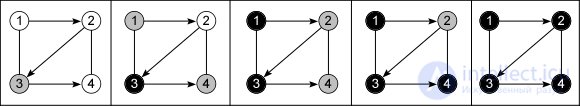
We have a mixed graph (see fig.) With | V | = 4 and | E | = 5. Perform a traversal of its vertices using a wide search algorithm. We take node 3 as the starting vertex. First, it is marked gray as detected, and then black, because nodes adjacent to it (1 and 4) are found, which, in turn, are marked in gray in the specified order. Next, node 1 is painted black, and its neighbors are located — node 2, which turns gray. And, finally, nodes 4 and 2, in this order, are viewed, and the wide bypass is completed.
The wide search algorithm works on both directed and undirected graphs. The mixed graph used in the example was intended to make this clear. It is worth noting that in an undirected connected graph, this method will bypass all the existing nodes, and in a mixed or digraph this will not necessarily happen. In addition, so far, we have considered the traversal of all vertices, but it is quite likely that it will be sufficient, for example, to view a certain number of them, or to find a particular vertex. In this case, it is necessary to adjust the algorithm a little, and not to change it completely or completely refuse to use it.
We now turn to a more formal description of the search algorithm in width. The main objects - the three data structures involved in the program will be:
The first two structures have an integer data type, the last - a logical one. Visited vertices are added to the visited array, which will prevent looping, and the queue queue will store the nodes involved. Recall that the data structure "queue" works on the principle of "first come, first come out." Consider the process of traversing a graph broken into stages:
The search in width, starting from the starting vertex, gradually moves away from it further and further, passing level by level. It turns out that at the end of the algorithm, all the shortest paths from the initial vertex to each node accessible from it will be found.
To implement the algorithm in PL, you need: the ability to programmatically set the graph, as well as to have an idea of such a data structure as a queue.
| one 2 3 four five 6 7 eight 9 ten eleven 12 13 14 15 sixteen 17 18 nineteen 20 21 22 23 24 25 26 27 28 29 thirty 31 32 33 34 35 36 37 38 39 40 41 42 43 44 45 46 47 48 49 50 51 52 53 54 55 |
#include "stdafx.h"
#include using namespace std; const int n = 4; int i, j; // graph adjacency matrix int GM [n] [n] = { {0, 1, 1, 0}, {0, 0, 1, 1}, {1, 0, 0, 1}, {0, 1, 0, 0} }; // search wide void BFS (bool * visited, int unit) { int * queue = new int [n]; int count, head; for (i = 0; i count = 0; head = 0; queue [count ++] = unit; visited [unit] = true; while (head { unit = queue [head ++]; cout << unit + 1 << ""; for (i = 0; i if (GM [unit] [i] &&! visited [i]) { queue [count ++] = i; visited [i] = true; } } delete [] queue; } // main function void main () { setlocale (LC_ALL, "Rus"); int start; cout << "Starting Top >>"; cin >> start; bool * visited = new bool [n]; cout << "Graph adjacency matrix:" << endl; for (i = 0; i { visited [i] = false; for (j = 0; j cout << "" << GM [i] [j]; cout << endl; } cout << "Bypass order:"; BFS (visited, start-1); delete [] visited; system ("pause >> void"); } |
| one 2 3 four five 6 7 eight 9 ten eleven 12 13 14 15 sixteen 17 18 nineteen 20 21 22 23 24 25 26 27 28 29 thirty 31 32 33 34 35 36 37 38 39 40 41 42 43 44 45 46 47 48 49 50 51 52 53 54 55 56 57 |
program BreadthFirstSearch;
uses crt; const n = 4; type MassivInt = array [1..n, 1..n] of integer; MassivBool = array [1..n] of boolean; var i, j, start: integer; visited: MassivBool; {graph adjacency matrix} const GM: MassivInt = ( (0, 1, 1, 0), (0, 0, 1, 1), (1, 0, 0, 1), (0, 1, 0, 0)); {search wide} procedure BFS (visited: MassivBool; _unit: integer); var queue: array [1..n] of integer; count, head: integer; begin for i: = 1 to n do queue [i]: = 0; count: = 0; head: = 0; count: = count + 1; queue [count]: = _ unit; visited [_unit]: = true; while head begin head: = head + 1; _unit: = queue [head]; write (_unit, ''); for i: = 1 to n do begin if (GM [_unit, i] <> 0) and (not visited [i]) then begin count: = count + 1; queue [count]: = i; visited [i]: = true; end; end; end; end; {main program block} begin clrscr; write ('Starting vertex >>'); read (start); writeln ('Count adjacency matrix:'); for i: = 1 to n do begin visited [i]: = false; for j: = 1 to n do write ('', GM [i, j]); writeln; end; write ('Bypass order:'); BFS (visited, start); end. |
The two programs use the graph shown in the previous figure, more precisely, its adjacency matrix. Only one of 4 values can give in to input, since it is possible to specify only one of 4 available vertices as a start (programs do not provide incorrect input data):
| Input data | Output |
| one | 1 2 3 4 |
| 2 | 2 3 4 1 |
| 3 | 3 1 4 2 |
| four | 4 2 3 1 |
The graph is represented by an adjacency matrix, and as far as efficiency is concerned, this is not the best option, since the time spent on its bypass is estimated at O (| V | 2 ), and it can be reduced to O (| V | + | E |) using adjacency list.

Comments
To leave a comment
Algorithms
Terms: Algorithms