Lecture
As you know, programs consist of two parts - algorithms and data structures. In a good program, these components effectively complement each other. The selection and implementation of the data structure is as important as the procedures for processing the data. The method of organizing and accessing information is usually determined by the nature of the programmed task. Thus, it is important for a programmer to have at his disposal techniques suitable for different situations.
The degree of data type binding to its machine representation is inversely related to its abstraction. In other words, the more abstract the data types become, the more the conceptual idea of how this data is stored differs from the actual, actual way they are stored in computer memory. Simple types, for example, char or int , are closely related to their machine representation. For example, the machine representation of an integer value approximates well the corresponding programming concept. As they become more complex, data types become conceptually less similar to their machine equivalents. So, floating point real numbers are more abstract than integers. The actual representation of the type of float in the machine rather approximately corresponds to the representation of the average programmer about the real number. Even more abstract is the structure belonging to composite data types.
At the next level of abstraction, the purely physical aspects of the data fade into the background due to the introduction of the data engine to data, that is, the mechanism for storing and retrieving information. Essentially, the physical data is associated with an access mechanism that manages the handling of data from the program. This chapter is dedicated to data access mechanisms.
There are four access mechanisms:
Each of these methods makes it possible to solve problems of a particular class. These methods are essentially mechanisms that perform certain operations of storing and retrieving information transmitted to them based on the requests they receive. They all save and receive an element; here, an element means an information unit. This chapter shows how to create such access mechanisms in C. This illustrates some common programming techniques in C, including dynamic memory allocation and the use of pointers.

[1] Other names: store, stack memory, store memory, store type memory, store type storage device, stack storage device.
[2] Other names: chain list, list using pointers, list with links, list on pointers.
[3] Other names: binary search tree.
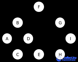
In computer science, a tree is a widely used abstract data type that simulates a hierarchical tree structure, with a root value and subtrees of children with a parent node, represented as a set of linked nodes.
A tree data structure can be defined recursively as a collection of nodes (starting at a root node), where each node is a data structure consisting of a value, together with a list of references to nodes (the "children"), with the constraints that no reference is duplicated, and none points to the root.
Alternatively, a tree can be defined abstractly as a whole (globally) as an ordered tree, with a value assigned to each node. Both these perspectives are useful: while a tree can be analyzed mathematically as a whole, when actually represented as a data structure it is usually represented and worked with separately by node (rather than as a set of nodes and an adjacency list of edges between nodes, as one may represent a digraph, for instance). For example, looking at a tree as a whole, one can talk about "the parent node" of a given node, but in general, as a data structure, a given node only contains the list of its children but does not contain a reference to its parent (if any).
A node is a structure which may contain a value or condition, or represent a separate data structure (which could be a tree of its own). Each node in a tree has zero or more child nodes, which are below it in the tree (by convention, trees are drawn growing downwards). A node that has a child is called the child's parent node (or superior). A node has at most one parent, but possibly many ancestor nodes, such as the parent's parent. Child nodes with the same parent are sibling nodes.
An internal node (also known as an inner node, inode for short, or branch node) is any node of a tree that has child nodes. Similarly, an external node (also known as an outer node, leaf node, or terminal node) is any node that does not have child nodes.
The topmost node in a tree is called the root node. Depending on the definition, a tree may be required to have a root node (in which case all trees are non-empty), or may be allowed to be empty, in which case it does not necessarily have a root node. Being the topmost node, the root node will not have a parent. It is the node at which algorithms on the tree begin, since as a data structure, one can only pass from parents to children. Note that some algorithms (such as post-order depth-first search) begin at the root, but first visit leaf nodes (access the value of leaf nodes), only visit the root last (i.e., they first access the children of the root, but only access the value of the root last). All other nodes can be reached from it by following edges or links. (In the formal definition, each such path is also unique.) In diagrams, the root node is conventionally drawn at the top. In some trees, such as heaps, the root node has special properties. Every node in a tree can be seen as the root node of the subtree rooted at that node.
The height of a node is the length of the longest downward path to a leaf from that node. The height of the root is the height of the tree. The depth of a node is the length of the path to its root (i.e., its root path). This is commonly needed in the manipulation of the various self-balancing trees, AVL Trees in particular. The root node has depth zero, leaf nodes have height zero, and a tree with only a single node (hence both a root and leaf) has depth and height zero. Conventionally, an empty tree (tree with no nodes, if such are allowed) has height −1.
A subtree of a tree T is a tree consisting of a node in T and all of its descendants in T.[a][1] Nodes thus correspond to subtrees (each node corresponds to the subtree of itself and all its descendants) – the subtree corresponding to the root node is the entire tree, and each node is the root node of the subtree it determines; the subtree corresponding to any other node is called a proper subtree (by analogy to a proper subset).
Other terms used with trees:
Neighbor
Parent or child.
Ancestor
A node reachable by repeated proceeding from child to parent.
Descendant
A node reachable by repeated proceeding from parent to child. Also known as subchild.
Branch node
Internal node
A node with at least one child.
Degree
For a given node, its number of children. A leaf has necessarily degree zero.
Degree of tree
The degree of a tree is the maximum degree of a node in the tree.
Distance
The number of edges along the shortest path between two nodes.
Level
1 + the number of edges between a node and the root, i.e. (depth + 1)[dubious – discuss]
Width
The number of nodes in a level.
Breadth
The number of leaves.
Forest
A set of n ≥ 0 disjoint trees.
Ordered tree
A rooted tree in which an ordering is specified for the children of each vertex.
Size of a tree
Number of nodes in the tree.
A tree is a nonlinear data structure, compared to arrays, linked lists, stacks and queues which are linear data structures. A tree can be empty with no nodes or a tree is a structure consisting of one node called the root and zero or one or more subtrees.
Trees are often drawn in the plane. Ordered trees can be represented essentially uniquely in the plane, and are hence called plane trees, as follows: if one fixes a conventional order (say, counterclockwise), and arranges the child nodes in that order (first incoming parent edge, then first child edge, etc.), this yields an embedding of the tree in the plane, unique up to ambient isotopy. Conversely, such an embedding determines an ordering of the child nodes.
If one places the root at the top (parents above children, as in a family tree) and places all nodes that are a given distance from the root (in terms of number of edges: the "level" of a tree) on a given horizontal line, one obtains a standard drawing of the tree. Given a binary tree, the first child is on the left (the "left node"), and the second child is on the right (the "right node").
Stepping through the items of a tree, by means of the connections between parents and children, is called walking the tree, and the action is a walk of the tree. Often, an operation might be performed when a pointer arrives at a particular node. A walk in which each parent node is traversed before its children is called a pre-order walk; a walk in which the children are traversed before their respective parents are traversed is called a post-order walk; a walk in which a node's left subtree, then the node itself, and finally its right subtree are traversed is called an in-order traversal. (This last scenario, referring to exactly two subtrees, a left subtree and a right subtree, assumes specifically a binary tree.) A level-order walk effectively performs a breadth-first search over the entirety of a tree; nodes are traversed level by level, where the root node is visited first, followed by its direct child nodes and their siblings, followed by its grandchild nodes and their siblings, etc., until all nodes in the tree have been traversed.
There are many different ways to represent trees; common representations represent the nodes as dynamically allocated records with pointers to their children, their parents, or both, or as items in an array, with relationships between them determined by their positions in the array (e.g., binary heap).
Indeed, a binary tree can be implemented as a list of lists (a list where the values are lists): the head of a list (the value of the first term) is the left child (subtree), while the tail (the list of second and subsequent terms) is the right child (subtree). This can be modified to allow values as well, as in Lisp S-expressions, where the head (value of first term) is the value of the node, the head of the tail (value of second term) is the left child, and the tail of the tail (list of third and subsequent terms) is the right child.
In general a node in a tree will not have pointers to its parents, but this information can be included (expanding the data structure to also include a pointer to the parent) or stored separately. Alternatively, upward links can be included in the child node data, as in a threaded binary tree.
If edges (to child nodes) are thought of as references, then a tree is a special case of a digraph, and the tree data structure can be generalized to represent directed graphs by removing the constraints that a node may have at most one parent, and that no cycles are allowed. Edges are still abstractly considered as pairs of nodes, however, the terms parent and child are usually replaced by different terminology (for example, source and target). Different implementation strategies exist: a digraph can be represented by the same local data structure as a tree (node with value and list of children), assuming that "list of children" is a list of references, or globally by such structures as adjacency lists.
In graph theory, a tree is a connected acyclic graph; unless stated otherwise, in graph theory trees and graphs are assumed undirected. There is no one-to-one correspondence between such trees and trees as data structure. We can take an arbitrary undirected tree, arbitrarily pick one of its vertices as the root, make all its edges directed by making them point away from the root node – producing an arborescence – and assign an order to all the nodes. The result corresponds to a tree data structure. Picking a different root or different ordering produces a different one.
Given a node in a tree, its children define an ordered forest (the union of subtrees given by all the children, or equivalently taking the subtree given by the node itself and erasing the root). Just as subtrees are natural for recursion (as in a depth-first search), forests are natural for corecursion (as in a breadth-first search).
Via mutual recursion, a forest can be defined as a list of trees (represented by root nodes), where a node (of a tree) consists of a value and a forest (its children):
f: [n[1], ..., n[k]]
n: v f
There is a distinction between a tree as an abstract data type and as a concrete data structure, analogous to the distinction between a list and a linked list.
As a data type, a tree has a value and children, and the children are themselves trees; the value and children of the tree are interpreted as the value of the root node and the subtrees of the children of the root node. To allow finite trees, one must either allow the list of children to be empty (in which case trees can be required to be non-empty, an "empty tree" instead being represented by a forest of zero trees), or allow trees to be empty, in which case the list of children can be of fixed size (branching factor, especially 2 or "binary"), if desired.
As a data structure, a linked tree is a group of nodes, where each node has a value and a list of references to other nodes (its children). There is also the requirement that no two "downward" references point to the same node. In practice, nodes in a tree commonly include other data as well, such as next/previous references, references to their parent nodes, or nearly anything.
Due to the use of references to trees in the linked tree data structure, trees are often discussed implicitly assuming that they are being represented by references to the root node, as this is often how they are actually implemented. For example, rather than an empty tree, one may have a null reference: a tree is always non-empty, but a reference to a tree may be null.
Recursively, as a data type a tree is defined as a value (of some data type, possibly empty), together with a list of trees (possibly an empty list), the subtrees of its children; symbolically:
t: v [t[1], ..., t[k]]
(A tree t consists of a value v and a list of other trees.)
More elegantly, via mutual recursion, of which a tree is one of the most basic examples, a tree can be defined in terms of forest (a list of trees), where a tree consists of a value and a forest (the subtrees of its children):
f: [t[1], ..., t[k]]
t: v f
Note that this definition is in terms of values, and is appropriate in functional languages (it assumes referential transparency); different trees have no connections, as they are simply lists of values.
As a data structure, a tree is defined as a node (the root), which itself consists of a value (of some data type, possibly empty), together with a list of references to other nodes (list possibly empty, references possibly null); symbolically:
n: v [&n[1], ..., &n[k]]
(A node n consists of a value v and a list of references to other nodes.)
This data structure defines a directed graph,[b] and for it to be a tree one must add a condition on its global structure (its topology), namely that at most one reference can point to any given node (a node has at most a single parent), and no node in the tree point to the root. In fact, every node (other than the root) must have exactly one parent, and the root must have no parents.
Indeed, given a list of nodes, and for each node a list of references to its children, one cannot tell if this structure is a tree or not without analyzing its global structure and that it is in fact topologically a tree, as defined below.
As an abstract data type, the abstract tree type T with values of some type E is defined, using the abstract forest type F (list of trees), by the functions:
value: T → E
children: T → F
nil: () → F
node: E × F → T
with the axioms:
value(node(e, f)) = e
children(node(e, f)) = f
In terms of type theory, a tree is an inductive type defined by the constructors nil (empty forest) and node (tree with root node with given value and children).
Viewed as a whole, a tree data structure is an ordered tree, generally with values attached to each node. Concretely, it is (if required to be non-empty):
together with:
Often trees have a fixed (more properly, bounded) branching factor (outdegree), particularly always having two child nodes (possibly empty, hence at most two non-empty child nodes), hence a "binary tree".
Allowing empty trees makes some definitions simpler, some more complicated: a rooted tree must be non-empty, hence if empty trees are allowed the above definition instead becomes "an empty tree or a rooted tree such that ...". On the other hand, empty trees simplify defining fixed branching factor: with empty trees allowed, a binary tree is a tree such that every node has exactly two children, each of which is a tree (possibly empty). The complete sets of operations on the tree must include fork operation.
Mathematically, an unordered tree[2] (or "algebraic tree")[3] can be defined as an algebraic structure (X, parent) where X is the non-empty carrier set of nodes and parent is a function on X which assigns each node x its "parent" node, parent(x). The structure is subject to the condition that every non-empty subalgebra must have the same fixed point. That is, there must be a unique "root" node r, such that parent(r) = r and for every node x, some iterative application parent(parent(⋯parent(x)⋯)) equals r.
There are several equivalent definitions.
As the closest alternative, one can define unordered trees as partial algebras (X, parent) which are obtained from the total algebras described above by letting parent(r) be undefined. That is, the root r is the only node on which the parent function is not defined and for every node x, the root is reachable from x in the directed graph (X, parent). This definition is in fact coincident with that of an anti-arborescence. The TAoCP book uses the term oriented tree.[4]
| An unordered tree is a structure (X, ≺) where X is a set of nodes and ≺ is a child-to-parent relation between nodes such that: | |
| (1) | X is non-empty. |
|---|---|
| (2) | X is weakly connected in ≺. |
| (3) | ≺ is functional. |
| (4) | ≺ satisfies ACC: there is no infinite sequence x1 ≺ x2 ≺ x3 ≺ ⋯. |
The box on the right describes the partial algebra (X, parent) as a relational structure (X, ≺). If (1) is replaced by
then condition (2) becomes redundant.
Using this definition, dedicated terminology can be provided for generalizations of unordered trees that correspond to distinguished subsets of the listed conditions:
Another equivalent definition of an unordered tree is that of a set-theoretic tree that is singly-rooted and whose height is at most ω (a "finite-ish" tree).[5] That is, the algebraic structures (X, parent) are equivalent to partial orders (X, ≤) that have a top element r and whose every principal upset (aka principal filter) is a finite chain. To be precise, we should speak about an inverse set-theoretic tree since the set-theoretic definition usually employs opposite ordering.
The correspondence between (X, parent) and (X, ≤) is established via reflexive transitive closure / reduction, with the reduction resulting in the "partial" version without the root cycle.
The definition of trees in descriptive set theory (DST) utilizes the representation of partial orders (X, ≥) as prefix orders between finite sequences. In turns out that up to isomorphism, there is a one-to-one correspondence between the (inverse of) DST trees and the tree structures defined so far.
We can refer to the four equivalent characterizations as to tree as an algebra, tree as a partial algebra, tree as a partial order, and tree as a prefix order. There is also a fifth equivalent definition – that of a graph-theoretic rooted tree which is just a connected acyclic rooted graph.
The expression of trees as (partial) algebras (also called functional graphs) (X, parent) follows directly the implementation of tree structures using parent pointers. Typically, the partial version is used in which the root node has no parent defined. However, in some implementations or models even the parent(r) = r circularity is established. Notable examples:
from object-oriented programming. In this case, the root node is the top metaclass – the only class that is a direct instance of itself.
Note that the above definition admits infinite trees. This allows for the description of infinite structures supported by some implementations via lazy evaluation. A notable example is the infinite regress of eigenclasses from the Ruby object model.[10] In this model, the tree established via superclass links between non-terminal objects is infinite and has an infinite branch (a single infinite branch of "helix" objects – see the diagram).
In every unordered tree (X, parent) there is a distinguished partition of the set X of nodes into sibling sets. Two non-root nodes x, y belong to the same sibling set if parent(x) = parent(y). The root node r forms the singleton sibling set {r}.[c] A tree is said to be locally finite or finitely branching if each of its sibling sets is finite.
Each pair of distinct siblings is incomparable in ≤. This is why the word unordered is used in the definition. Such a terminology might become misleading when all sibling sets are singletons, i.e. when the set X of all nodes is totally ordered (and thus well-ordered) by ≤ In such a case we might speak about a singly-branching tree instead.
As with every partially ordered set, tree structures (X, ≤) can be represented by inclusion order – by set systems in which ≤ is coincident with ⊆, the induced inclusion order. Consider a structure (U, ℱ) such that U is a non-empty set, and ℱ is a set of subsets of U such that the following are satisfied (by Nested Set Collection definition):
Then the structure (ℱ, ⊆) is an unordered tree whose root equals U. Conversely, if (U, ≤) is an unordered tree, and ℱ is the set {↓x | x ∈ U} of all principal ideals of (U, ≤) then the set system (U, ℱ) satisfies the above properties.
The set-system view of tree structures provides the default semantic model – in the majority of most popular cases, tree data structures represent containment hierarchy. This also offers a justification for order direction with the root at the top: The root node is a greater container than any other node. Notable examples:
An unordered tree (X, ≤) is well-founded if the strict partial order < is a well-founded relation. In particular, every finite tree is well-founded. Assuming the axiom of dependent choice a tree is well-founded if and only if it has no infinite branch.
Well-founded trees can be defined recursively – by forming trees from a disjoint union of smaller trees. For the precise definition, suppose that X is a set of nodes. Using the reflexivity of partial orders, we can identify any tree (Y, ≤) on a subset of X with its partial order (≤) – a subset of X × X. The set ℛ of all relations R that form a well-founded tree (Y, R) on a subset Y of X is defined in stages ℛi, so that ℛ = ⋃{ℛi | i is ordinal}. For each ordinal number i, let R belong to the i-th stage ℛi if and only if R is equal to
⋃ℱ ∪ ((dom(⋃ℱ) ∪ {x}) × {x})
where ℱ is a subset of ⋃{ℛk | k < i} such that elements of ℱ are pairwise disjoint, and x is a node that does not belong to dom(⋃ℱ). (We use dom(S) to denote the domain of a relation S.) Observe that the lowest stage ℛ0 consists of single-node trees {(x,x)} since only empty ℱ is possible. In each stage, (possibly) new trees R are built by taking a forest ⋃ℱ with components ℱ from lower stages and attaching a new root x atop of ⋃ℱ.
In contrast to the tree height which is at most ω, the rank of well-founded trees is unlimited,[12] see the properties of "unfolding".
In computing, a common way to define well-founded trees is via recursive ordered pairs (F, x): a tree is a forest F together with a "fresh" node x.[13] A forest F in turn is a possibly empty set of trees with pairwise disjoint sets of nodes. For the precise definition, proceed similarly as in the construction of names used in the set-theoretic technique of forcing. Let X be a set of nodes. In the superstructure over X, define sets T, ℱ of trees and forests, respectively, and a map nodes : T → ℘(X) assigning each tree t its underlying set of nodes so that:
| (trees over X) | t ∈ T | ↔ | t is a pair (F, x) from ℱ × X such that for all s ∈ F, x ∉ nodes(s), |
|
| (forests over X) | F ∈ ℱ | ↔ | F is a subset of T such that for every s,t ∈ F, s ≠ t, nodes(s) ∩ nodes(t) = ∅ }}, |
|
| (nodes of trees) | y ∈ nodes(t) | ↔ | t = (F, x) ∈ T and either y = x or y ∈ nodes(s) for some s ∈ F }}. |
Circularities in the above conditions can be eliminated by stratifying each of T, ℱ and nodes into stages like in the previous subsection. Subsequently, define a "subtree" relation ≤ on T as the reflexive transitive closure of the "immediate subtree" relation ≺ defined between trees by
| s ≺ t | ↔ | s ∈ π1(t) |
where π1(t) is the projection of t onto the first coordinate; i.e., it is the forest F such that t = (F, x) for some x ∈ X. It can be observed that (T, ≤) is a multitree: for every t ∈ T, the principal ideal ↓t ordered by ≤ is a well-founded tree as a partial order. Moreover, for every tree t ∈ T, its "nodes"-order structure (nodes(t), ≤t) is given by x ≤t y if and only if there are forests F, G ∈ ℱ such that both (F, x) and (G, y) are subtrees of t and (F, x) ≤ (G, y).
Another formalization as well as generalization of unordered trees can be obtained by reifying parent-child pairs of nodes. Each such ordered pair can be regarded as an abstract entity – an "arrow". This results in a multidigraph (X, A, s, t) where X is the set of nodes, A is the set of arrows, and s and t are functions from A to X assigning each arrow its source and target, respectively. The structure is subject to the following conditions:
In (1), the composition symbol ○ is to be interpreted left-to-right. The condition says that inverse consecutivity of arrows[d] is a total child-to-parent map. Let this parent map between arrows be denoted p, i.e. p = s ○ t−1. Then we also have s = p ○ t, thus a multidigraph satisfying (1,2) can also be axiomatized as (X, A, p, t), with the parent map p instead of s as a definitory constituent. Observe that the root arrow is necessarily a loop, i.e. its source and target coincide.

An important generalization of the above structure is established by allowing the target map t to be many-to-one. This means that (2) is weakened to
(2') The t map is surjective – each node is the target of some arrow.
Note that condition (1) asserts that only leaf arrows are allowed to have the same target. That is, the restriction of t to the range of p is still injective.
Multidigraphs satisfying (1,2') can be called "arrow trees" – their tree characteristics is imposed on arrows rather than nodes. These structures can be regarded as the most essential abstraction of the Linux VFS because they reflect the hard-link structure of filesystems. Nodes are called inodes, arrows are dentries (or hard links). The parent and target maps p and t are respectively represented by d_parent and d_inode fields in the dentry data structure.[14] Each inode is assigned a fixed file type, of which the directory type plays a special role of "designed parents":
Using dashed style for the first half of the root loop indicates that, similarly to the parent map, there is a partial version for the source map s in which the source of the root arrow is undefined. This variant is employed for further generalization, see #Using paths in a multidigraph.
Unordered trees naturally arise by "unfolding" of accessible pointed graphs.[15]
Let ℛ = (X, R, r) be a pointed relational structure, i.e. such that X is the set of nodes, R is a relation between nodes (a subset of X × X), and r is a distinguished "root" node. Assume further that ℛ is accessible, which means that X equals the preimage of {r} under the reflexive transitive closure of R, and call such a structure an accessible pointed graph or apg for short.(⁎) Then one can derive another apg ℛ' = (X', R', r') – the unfolding of ℛ – as follows:
Apparently, the structure (X', R') is an unordered tree in the "partial-algebra" version: R' is a partial map that relates each non-root element of X' to its parent by path popping. The root element is obviously r'. Moreover, the following properties are satisfied:
Notes:
(⁎) To establish a concordancy between R and the parent map, the presented definition uses reversed accessibility: r is reachable from any node. In the original definition by P. Aczel[15], every node is reachable from r (thus, instead of "preimage", the word "image" applies).[e]
(⁑) We have implicitly introduced a definition of unordered trees as apgs: call an apg ℛ = (X, R, r) a tree if the reduct (X, R) is an unordered tree as a partial algebra. This can be translated as: Every node is accessible by exactly one path.
As shown on the example of hard-link structure of file systems, many data structures in computing allow multiple links between nodes. Therefore, in order to properly exhibit the appearance of unordered trees among data structures it is necessary to generalize accessible pointed graphs to multidigraph setting. To simplify the terminology, we make use of the term quiver which is an established synonym for "multidigraph".
Let an accessible pointed quiver or apq for short be defined as a structure
ℳ = (X, A, s, t)
where
X is a set of nodes,
A is a set of arrows,
s is a partial function from A to X (the source map), and
t is a total function from A to X (the target map).
Thus, ℳ is a "partial multidigraph".
The structure is subject to the following conditions:
ℳ is said to be a tree if the target map t is a bijection between arrows and nodes. The unfolding of ℳ is formed by the sequences mentioned in (2) – which are the accessibility paths (cf. Path algebra). As an apq, the unfolding can be written as
ℳ' = (X', A', s', t')
where
X' is the set of accessibility paths,
A' coincides with X',
s' coincides with path popping, and
t' is the identity on X'.
Like with apgs, unfolding is idempotent and always results in a tree.
The underlying apg is obtained as the structure
(X, R, t(ar))
where
R = {(t(a),s(a)) | a ∈ A \ {ar}}.
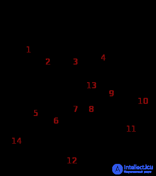
The diagram above shows an example of an apq with 1 + 14 arrows. In JavaScript, Python or Ruby, the structure can be created by the following (exactly the same) code:
r = {};
r[1] = {}; r[2] = r[1]; r[3] = {}; r[4] = {};
r[1][5]    = {};   r[1][14]    = r[1][5];
r[3][7]    = {};   r[3][8]     = r[3][7];  r[3][13] = {};
r[4][9]    = r[4]; r[4][10]    = r[4];     r[4][11] = {};
r[3][7][6] = r[3]; r[3][7][12] = r[1][5];
Unordered trees and their generalizations form the essence of naming systems. There are two prominent examples of naming systems: file systems and (nested) associative arrays. The multidigraph-based structures from previous subsections provided anonymous abstractions for both cases. To obtain naming capabilities, arrows are to be equipped with names as identifiers. A name must be locally unique – within each sibling set of arrows[f] there can be at most one arrow labelled by a given name.
source |
name |
target |
|---|---|---|
| s(a) | σ(a) | t(a) |
This can be formalized as a structure
ℰ = (X, Σ, A, s, σ, t)
where
X is a set of nodes,
Σ is a set of names,
A is a set of arrows,
s is a partial function from A to X,
σ is a partial function from A to Σ, and
t is a total function from A to X.
For an arrow a, constituents of the triple (s(a), σ(a), t(a)) are respectively a's source, name and target. The structure is subject to the following conditions:
This structure can be called a nested dictionary or named apq. In computing, such structures are ubiquitous. The table above shows that arrows can be considered "un-reified" as the set A' = {(s(a), σ(a), t(a)) | a ∈ A \ {ar}} of source-name-target triples. This leads to a relational structure (X, Σ, A') which can be viewed as a relational database table. Underlines in source and name indicate primary key.
The structure can be rephrased as a deterministic labelled transition system: X is a set of "states", Σ is a set of "labels", A' is a set of "labelled transitions". (Moreover, the root node r = t(ar) is an "initial state", and the accessibility condition means that every state is reachable from the initial state.)
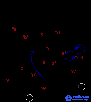
The diagram on the right shows a nested dictionary ℰ that has the same underlying multidigraph as the example in the previous subsection. The structure can be created by the code below. Like before, exactly the same code applies for JavaScript, Python and Ruby.
First, a substructure, ℰ0, is created by a single assignment of a literal {...} to r. This structure, depicted by full lines, is an "arrow tree" (therefore, it is a spanning tree). The literal in turn appears to be a JSON serialization of ℰ0.
Subsequently, the remaining arrows are created by assignments of already existing nodes. Arrows that cause cycles are displayed in blue.
r = {"a":{"a":5,"b":5},"c":{"a":{"w":5},"c":{}},"d":{"w":1.3}}

r["b"]           = r["a"]; r["c"]["b"] = r["c"]["a"]
r["c"]["a"]["p"] = r["c"]; r["d"]["e"] = r["d"]["self"] = r["d"]
In the Linux VFS, the name function σ is represented by the d_name field in the dentry data structure.[14] The ℰ0 structure above demonstrates a correspondence between JSON-representable structures and hard-link structures of file systems. In both cases, there is a fixed set of built-in types of "nodes" of which one type is a container type, except that in JSON, there are in fact two such types – Object and Array. If the latter one is ignored (as well as the distinction between individual primitive data types) then the provided abstractions of file-systems and JSON data are the same – both are arrow trees equipped with naming σ and a distinction of container nodes.
The naming function σ of a nested dictionary ℰ naturally extends from arrows to arrow paths. Each sequence p = [a1, ..., an] of consecutive arrows is implicitly assigned a pathname (cf. Pathname) – the sequence σ(p) = [σ(a1), ..., σ(an)] of arrow names.[g] Local uniqueness carries over to arrow paths: different sibling paths have different pathnames. In particular, the root-originating arrow paths are in one-to-one correspondence with their pathnames. This correspondence provides a "symbolic" representation of the unfolding of ℰ via pathnames – the nodes in ℰ are globally identified via a tree of pathnames.
The structures introduced in the previous subsection form just the core "hierarchical" part of tree data structures that appear in computing. In most cases, there is also an additional "horizontal" ordering between siblings. In search trees the order is commonly established by the "key" or value associated with each sibling, but in many trees that is not the case. For example, XML documents, lists within JSON files, and many other structures have order that does not depend on the values in the nodes, but is itself data — sorting the paragraphs of a novel alphabetically would lose information.[dubious – discuss]
The correspondent expansion of the previously described tree structures (X, ≤) can be defined by endowing each sibling set with a linear order as follows.[17][18]
An alternative definition according to Kuboyama[2] is presented in the next subsection.
An ordered tree is a structure (X, ≤V, ≤S) where X is a non-empty set of nodes and ≤V and ≤S are relations on X called vertical (or also hierarchical[2]) order and sibling order, respectively. The structure is subject to the following conditions:
(<S) ∪ (>S) = ((≺V) ○ (≻V)) ∖ idX.
Conditions (2) and (3) say that (X, ≤S) is a component-wise linear order, each component being a sibling set. Condition (4) asserts that if a sibling set S is infinite then (S, ≤S) is isomorphic to (ℕ, ≤), the usual ordering of natural numbers.
Given this, there are three (another) distinguished partial orders which are uniquely given by the following prescriptions:
| (<H) | = | (≤V) ○ (<S) ○ (≥V) | (the horizontal order), |
| (<L⁻) | = | (>V) ∪ (<H) | (the "discordant" linear order), |
| (<L⁺) | = | (<V) ∪ (<H) | (the "concordant" linear order). |
This amounts to a "V-S-H-L±" system of five partial orders ≤V, ≤S, ≤H, ≤L⁺, ≤L⁻ on the same set X of nodes, in which, except for the pair { ≤S, ≤H }, any two relations uniquely determine the other three, see the determinacy table.
Notes about notational conventions:
 ).
).This yields six versions ≺, <, ≤, ≻, >, ≥ for a single partial order relation. Except for ≺ and ≻, each version uniquely determines the others. Passing from ≺ to <requires that < be transitively reducible. This is always satisfied for all of <V, <S and <H but might not hold for <L⁺ or <L⁻ if X is infinite.
The partial orders ≤V and ≤Hare complementary:
(<V) ⊎ (>V) ⊎ (<H) ⊎ (>H) = X × X ∖ idX.
As a consequence, the "concordant" linear order <L⁺ is a linear extension of <V. Similarly, <L⁻ is a linear extension of >V.
The covering relations ≺L⁻ and ≺L⁺ correspond to pre-order traversal and post-order traversal, respectively. If x ≺L⁻ y then, according to whether y has a previous sibling or not, the x node is either the "rightmost" non-strict descendant of the previous sibling of y or, in the latter case, x is the first child of y. Pairs  of the latter case form the relation (≺L⁻) ∖ (<H) which is a partial map that assigns each non-leaf node its first child node. Similarly, (≻L⁺) ∖ (>H) assigns each non-leaf node with finitely many children its last child node.
The Kuboyama's definition of "rooted ordered trees"[2] makes use of the horizontal order ≤H as a definitory relation.[h] (See also Suppes.[19])
Using the notation and terminology introduced so far, the definition can be expressed as follows.
An ordered tree is a structure (X, ≤V, ≤H) such that conditions (1–5) are satisfied:
(That is, pairs of nodes that are incomparable in (<V) are comparable in (<H) and vice versa.)
(That is, for every nodes x, y such that x <H y, all descendants of x must precede all the descendants of y.)
The sibling order (≤S) is obtained by (<S) = (<H) ∩ ((≺V) ○ (≻V)), i.e. two distinct nodes are in sibling order if and only if they are in horizontal order and are siblings.
The following table shows the determinacy of the "V-S-H-L±" system. Relational expressions in the table's body are equal to one of <V, <S, <H, <L⁻, or <L⁺ according to the column. It follows that except for the pair { ≤S, ≤H }, an ordered tree (X, ...) is uniquely determined by any two of the five relations.
| <V | <S | <H | <L⁻ | <L⁺ | |
|---|---|---|---|---|---|
| V,S | (≤V) ○ (<S) ○ (≥V) | ||||
| V,H | (<H) ∩ ((≺V)○(≻V)) | (>V) ∪ (<H) | (<V) ∪ (<H) | ||
| V,L⁻ | (<L⁻) ∩ ((≺V)○(≻V)) | (<L⁻) ∖ (>V) | |||
| V,L⁺ | (<L⁺) ∩ ((≺V)○(≻V)) | (<L⁺) ∖ (<V) | |||
| H,L⁻ | (>L⁻) ∖ (<H) | ||||
| H,L⁺ | (<L⁺) ∖ (<H) | ||||
| L⁻,L⁺ | (>L⁻) ∩ (<L⁺) | (<L⁻) ∩ (<L⁺) | |||
| S,L⁻ | x ≺V y ↔ y = infL⁻(Y) where Y is the image of {x} under (≥S)○(≻L⁻) | ||||
| S,L⁺ | x ≺V y ↔ y = supL⁺(Y) where Y is the image of {x} under (≤S)○(≺L⁺) | ||||
In the last two rows, infL⁻(Y) denotes the infimum of Y in (X, ≤L⁻), and supL⁺(Y) denotes the supremum of Y in (X, ≤L⁺). In both rows, (≤S) resp. (≥S) can be equivalently replaced by the sibling equivalence (≤S)○(≥S). In particular, the partition into sibling sets together with either of ≤L⁻ or ≤L⁺ is also sufficient to determine the ordered tree. The first prescription for ≺V can be read as: the parent of a non-root node x equals the infimum of the set of all immediate predecessors of siblings of x, where the words "infimum" and "predecessors" are meant with regard to ≤L⁻. Similarly with the second prescription, just use "supremum", "successors" and ≤L⁺.
The relations ≤S and ≤H obviously cannot form a definitory pair. For the simplest example, consider an ordered tree with exactly two nodes – then one cannot tell which of them is the root.
| XPath axis | Relation |
|---|---|
ancestor |
<V |
ancestor-or-self |
≤V |
child |
≻V |
descendant |
>V |
descendant-or-self |
≥V |
following |
<H |
following-sibling |
<S |
parent |
≺V |
preceding |
>H |
preceding-sibling |
>S |
self |
idX |
The table on the right shows a correspondence of introduced relations to XPath axes, which are used in structured document systems to access nodes that bear particular ordering relationships to a starting "context" node. For a context node[20] x, its axis named by the specifier in the left column is the set of nodes that equals the image of {x} under the correspondent relation. As of XPath 2.0, the nodes are "returned" in document order, which is the "discordant" linear order ≤L⁻. A "concordance" would be achieved, if the vertical order ≤V was defined oppositely, with the bottom-up direction outwards the root like in set theory in accordance to natural trees.[i]
Below is the list of partial maps that are typically used for ordered tree traversal.[21] Each map is a distinguished functional subrelation of ≤L⁻ or of its opposite.
The traversal maps constitute a partial unary algebra[22] (X, parent, previousSibling, ..., nextNode) that forms a basis for representing trees as linked data structures. At least conceptually,there are parent links, sibling adjacency links, and first / last child links. This also applies to unordered trees in general, which can be observed on the dentry data structure in the Linux VFS.[23]
Similarly to the "V-S-H-L±" system of partial orders, there are pairs of traversal maps that uniquely determine the whole ordered tree structure. Naturally, one such generating structure is (X, V, S) which can be transcribed as (X, parent, nextSibling) – the structure of parent and next-sibling links. Another important generating structure is (X, firstChild, nextSibling) known as left-child right-sibling binary tree. This partial algebra establishes a one-to-one correspondence between binary trees and ordered trees.
The correspondence to binary trees provides a concise definition of ordered trees as partial algebras.
An ordered tree is a structure  where X is a non-empty set of nodes, and lc, rs are partial maps on X called left-child and right-sibling, respectively. The structure is subject to the following conditions:
The partial order structure (X, ≤V, ≤S) is obtained as follows:
| (≺S) | = | (rs), |
| (≻V) | = | (lc) ○ (≤S). |
Ordered trees can be naturally encoded by finite sequences of natural numbers.[24][j] Denote ω⁎ the set of all finite sequences of natural numbers. Then any non-empty subset W of ω⁎ that is closed under taking prefixes gives rise to an ordered tree: take the prefix order for ≥V and the lexicographical order for ≤L⁻. Conversely, for an ordered tree T = (X, V, ≤L⁻) assign each node x the sequence  of sibling indices, i.e. the root is assigned the empty sequence and for every non-root node x, let w(x) = w(parent(x)) ⁎ [i] where i is the number of preceding siblings of x and ⁎ is the concatenation operator. Put W = {w(x) | x ∈ X}. Then W, equipped with the induced orders ≤V (the inverse of prefix order) and ≤L⁻ (the lexicographical order), is isomorphic to T.
As a possible expansion of the "V-S-H-L±" system, another distinguished relations between nodes can be defined, based on the tree's level structure. First, let us denote by ∼E the equivalence relation defined by x ∼E y if and only if x and y have the same number of ancestors. This yields a partition of the set of nodes into levels L0, L1, ... (, Ln) – a coarsement of the partition into sibling sets. Then define relations <E, <B⁻ and <B⁺ by

It can be observed that <E is a strict partial order and <B⁻ and <B⁺ are strict total orders. Moreover, there is a similarity between the "V-S-L±" and "V-E-B±" systems: <E is component-wise linear and orthogonal to <V, <B⁻ is linear extension of <E and of >V, and <B⁺ is a linear extension of <E and of <V.


Comments
To leave a comment
Structures and data processing algorithms.
Terms: Structures and data processing algorithms.