Lecture
The data structures and algorithms are the materials from which the programs are built. Moreover, the computer itself consists of data structures and algorithms. The embedded data structures are represented by those registers and memory words where binary values are stored. The algorithms embedded in the hardware design are strict rules embodied in electronic logic circuits, according to which memorized data are interpreted as commands to be executed. Therefore, the basis of any computer is the ability to operate with only one type of data - with individual bits, or binary digits. The computer works with this data only in accordance with the invariable set of algorithms, which are determined by the system of commands of the central processor.
Tasks that are solved with the help of a computer are rarely expressed in the language of bits. As a rule, data is in the form of numbers, letters, texts, symbols, and more complex structures such as sequences, lists, and trees. The algorithms used to solve various problems are even more diverse; in fact, algorithms are not less than computational problems.
For an accurate description of abstract data structures and program algorithms, such formal notation systems are used, called programming languages, in which the meaning of any sentence is defined precisely and unambiguously. Among the tools provided by almost all programming languages, it is possible to refer to a data element using the name assigned to it, or, otherwise, the identifier. Some named values are constants that retain a constant value in the part of the program where they are defined, others are variables to which any new value can be assigned by the operator in the program. But until the program starts to run, their value is undefined.
The name of a constant or variable helps the programmer, but it doesn’t say anything to the computer. The compiler, translating the program text into binary code, associates each identifier with a specific memory address. But in order for the compiler to do this, you need to report the “type” of each named value. A person who solves any problem "manually" has an intuitive ability to quickly understand the types of data and those operations that are true for each type. For example, you can not extract the square root of a word or write a number with a capital letter. One of the reasons for making such recognition easy is that words, numbers, and other designations look different. However, for a computer, all data types ultimately boil down to a sequence of bits, so the difference in types should be made explicit.
Data types accepted in programming languages include natural and integer numbers, real (real) numbers (in the form of approximate decimal fractions), letters, strings, etc.
In some programming languages, the type of each constant or variable is determined by the compiler by writing the assigned value; the presence of a decimal point, for example, can be a sign of a real number. Other languages require the programmer to explicitly specify the type of each variable, and this gives one important advantage. Although the value of a variable can change many times during program execution, its type should never change; this means that the compiler can check the operations performed on this variable and make sure that they all agree with the description of the type of the variable. Such verification can be carried out by analyzing the entire program text, and in this case it will cover all possible actions determined by this program.
Depending on the purpose of the programming language, type protection performed at the compilation stage may be more or less rigid. Thus, for example, the PASCAL language, which was originally primarily a tool for illustrating data structures and algorithms, retains a very strict type protection from its original purpose. In most cases, the PASCAL compiler regards the mixing of data of different types in one expression or the application of uncharacteristic operations to the data type as a fatal error. In contrast, the C language, intended primarily for system programming, is a language with very weak type protection. C-compilers in such cases only give warnings. The absence of strict type protection gives the system programmer developing a C program additional possibilities, but such a programmer is responsible for the correctness of his actions.
The data structure refers essentially to "spatial" concepts: it can be reduced to a scheme for organizing information in a computer's memory. The algorithm is the corresponding procedural element in the program structure - it serves as a recipe for calculation.
The first algorithms were invented to solve numerical problems such as multiplying numbers, finding the greatest common divisor, calculating trigonometric functions, and others. Today, unnumbered algorithms are equally important; they are designed for tasks such as, for example, searching a specific word in a text, planning events, sorting data in a specified order, and so on. Unnumbered algorithms operate on data that is not necessarily a number; moreover, no deep mathematical concepts are needed to construct or understand them. From this, however, it does not at all follow that there is no place for mathematics in the study of such algorithms; on the contrary, exact mathematical methods are needed when searching for the best solutions to non-numerical problems in proving the correctness of these solutions.
The data structures used in the algorithms can be extremely complex. As a result, choosing the right data representation is often the key to successful programming and can have a greater effect on program performance than the details of the algorithm used. Hardly ever there will be a general theory of a choice of data structures. The best thing you can do is to understand all the basic “bricks” and the structures assembled from them. The ability to apply this knowledge to the design of large systems is primarily a matter of engineering skill and practice.
Beginning the study of data structures or information structures, it is necessary to clearly establish what is meant by information, how information is transmitted and how it is physically located in the memory of the computer.
It can be said that solving each task with the help of a computer involves recording information into memory, retrieving information from memory, and manipulating information. Is it possible to measure information?
In the theoretical information sense, information is considered as a measure for resolving uncertainty. Suppose that there are n possible states of some system in which each state has a probability of occurrence p, and all probabilities are independent. Then the uncertainty of this system is defined as
  n
                  H = - SUM (p (i) * log2 (p (i))).
                         i = 1
To measure the uncertainty of the system, a special unit is chosen, called a bit. A bit is a measure of the uncertainty (or information) associated with the presence of only two possible states, such as, for example, true-false or yes-no. The bit is used to measure both uncertainty and information. This is understandable, since the amount of information received is equal to the amount of uncertainty eliminated as a result of receiving information.
In digital computers, there are three main types of storage devices: super-operative, operative and external memory. Usually, super-operative memory is built on registers. Registers are used for temporary storage and conversion of information.
Some of the most important registers are contained in the central processor of the computer. The central processor contains registers (sometimes called batteries) in which the arguments (ie, operands) of arithmetic operations are placed. Addition, subtraction, multiplication and division of the information stored in the batteries is performed using very complex logic circuits. In addition, individual bits can be analyzed to verify the need to change the normal control gear sequence in batteries. In addition to memorizing operands and the results of arithmetic operations, registers are also used to temporarily store program instructions and control information about the number of the next instruction being executed.
RAM is designed to memorize more permanent information in its nature. The most important property of RAM is addressability. This means that each memory cell has its own identifier, which uniquely identifies it in the general array of memory cells. This identifier is called an address. Cell addresses are operands of those machine instructions that access RAM. In the overwhelming majority of modern computing systems, the unit of addressing is a byte — a cell consisting of 8 binary bits. A specific memory cell or multiple cells can be associated with a specific variable in the program. However, to perform arithmetic calculations in which a variable participates, it is necessary that, prior to the beginning of the calculations, the value of the variable is transferred from the memory cell to the register. If the result of the calculation must be assigned to a variable, then the resulting value must again be transferred from the corresponding register to the memory cell associated with this variable.
During the execution of the program, its commands and data are mainly located in memory cells. The full array of memory elements is often referred to as main memory.
External memory serves primarily for long-term data storage. Characteristic for data on external memory is that they can be stored there even after the program that created them is completed and can be subsequently reused by the same program when it is restarted or by other programs. External memory is also used to store the programs themselves when they are not executed. Since the cost of external memory is much less than operational memory, and the amount is much larger, another purpose of external memory is to temporarily store those codes and data of the program being executed that are not used at this stage of its execution. The active codes of the program being executed and the data processed by it at this stage must necessarily be placed in RAM, since direct exchange between external memory and operational devices (registers) is impossible.
As a data warehouse, external memory has basically the same properties as operational memory, including the addressability property. Therefore, in principle, the data structures on external memory can be the same as in operational memory, and the algorithms for their processing can be the same. But external memory has a completely different physical nature, different access methods are used for it (on the physical level), and this access has other temporal characteristics. This leads to the fact that the structures and algorithms that are effective for RAM, are not so for external memory.
To provide an appropriate basis for studying data structures, existing types of number systems should be discussed: positional and non-positional.
Numbers are used to symbolically represent the number of objects. A very simple method of representing quantities is to use the same icons. In such a system, a one-to-one correspondence is established between the icons and the recalculated objects. For example, six objects can be represented as ****** or 111111. Such a system becomes very inconvenient if you try to use it to present large quantities.
Number systems like the Roman ones provide a partial solution to the problem of representing a large number of objects. In the Roman system, additional symbols serve to represent groups of icons. For example, you can accept that I = *, Y = IIIII, X = YY, L = XXXXX, etc. The specified value is represented by combining characters in accordance with a number of rules, which to some extent depend on the position of the character in the number. The disadvantage of the system, which from the very beginning is based on the grouping of a certain set of symbols in order to form a new symbol, is the fact that to represent very large numbers a lot of unique symbols are required.
In the positional number system uses a finite number of R unique characters. The value of R is often called the base of the number system. In a positional system, a quantity is represented both by the characters themselves and by their position in the number record.
The number system with a base of ten, or the decimal system is positional. Consider, for example, the number 1303. It can be represented as:
1 * 10 ^ 3 + 3 * 10 ^ 2 + 0 * 10 ^ 1 + 3 * 10 ^ 0.
(Hereinafter, the ^ symbol is used as a sign of exponentiation operation).
In the positional system can be represented and fractional numbers. For example, one-fourth is written as 0.25, which is interpreted as:
2 * 10 ^ (- 1) + 5 * 10 ^ (- 2).
Another example of a positional number system is the binary system. The binary number 11001.101 represents the same amount as the decimal number 26.625. The decomposition of this binary number in accordance with its positional representation is as follows:
  1 * 2 ^ 4 + 1 * 2 ^ 3 + 0 * 2 ^ 1 + 1 * 2 ^ 0 + 1 * 2 ^ (- 1) + 0 * 2 ^ (- 2) + 1 * 2 ^ (- 3) =
        16 + 8 + 1 + 0.5 + 0.125 = 26.625.
The most common numbering systems have a base of 2,8,10 and 16, which are usually called binary, octal, decimal and hexadecimal systems, respectively. All computing equipment operates in a binary number system, since the basic elements of computing equipment have two stable states. The octal and hexadecimal systems are used for the convenience of working with large binary numbers.
The image of numbers in any positional number system with a natural base R (R> 1) is based on representing them as a product of integer degree m of base R by a polynomial from this base:
  n
                   Ar = R ^ m * SUM (a [i] * R ^ (- i)), (1.1)
                               i = 1
Where:
Thus, in the decimal (R = 10) system, the numbers are used to represent numbers a = {0,1, ... 9}; in binary (R = 2) - a = {0,1}, in hexadecimal (R = 16), a = {0,1 .... 9, A, B, C, D, E, F} where uppercase Latin letters A..F are equivalent respectively to the numbers 10..15 in the decimal system. For example,
  1) 815 = 10 ^ 3 * (8 * 10 ^ (- 1) + 1 * 10 ^ (- 2) + 5 * 10 (-3) = 8 * 10 ^ 2 + 1 * 10 ^ 1 + 5 * 10 ^ 0;
 2) 8.15 = 10 ^ 1 * (8 * 10 ^ (- 1) + 1 * 10 ^ (- 2) + 5 * 10 ^ (- 3) = 8 * 10 ^ 0 + 1 * 10 ^ (- 1 ) + 5 * 10 ^ (- 2);
 3) 0.0815 = 10 ^ (- 1) * (8 * 10 ^ (- 1) + 1 * 10 ^ (- 2) + 5 * 10 ^ (- 3)) =
    = 8 * 10 ^ (- 2) + 1 * 10 ^ (- 3) + 5 * 10 ^ (- 4);
When translating an integer (the integer part of a number) from one number system to another, the original number (or the integer part) must be divided by the base of the number system into which the translation is made. Division to perform, while the private will not be less than the base of the new number system. The result of the transfer is determined by the remainder of the division: the first remainder gives the lower digit of the resulting number, the last quotient from the division gives the highest digit.
When translating the correct fraction from one number system to another number system, the fraction should be multiplied by the base of the number system into which the translation is made. The integer part obtained after the first multiplication is the highest digit of the resulting number. The multiplication is carried out until the product becomes zero or the required number of characters after the dividing point is not obtained.
For example,
  0.243 (10) ---> 0.0011111 (2).
      Check: 0.0011111 = 0 * 2 ^ (- 1) + 0 * 2 ^ (- 2) + 1 * 2 ^ (- 3) +
      1 * 2 ^ (- 4) + 1 * 2 ^ (- 5) + + 1 * 2 ^ (- 6) + 1 * 2 * (- 7) = 0.2421875
2) translate the integer 164 from the decimal number system into the binary system.
  164 (10) ---> 10100100 (2)
      Check: 10100100 = 1 * 2 ^ 7 + 0 * 2 ^ 6 + 1 * 2 ^ 5 + 0 * 2 ^ 4 +
      0 * 2 ^ 3 + 1 * 2 ^ 2 + 0 * 2 ^ 1 + 0 * 2 ^ 0 = 128 + 32 + 4 = 164
When translating mixed numbers, the integer and fractional parts of a number are translated separately.
Now it is possible to give a more specific definition of the information representation given at the machine level.
Regardless of the content and complexity, any data in the computer memory is represented by a sequence of binary digits, or bits, and their values are the corresponding binary numbers. The data, considered as a sequence of bits, have a very simple organization or, in other words, are weakly structured.For a person to describe and investigate any complex data in terms of sequences of bits is very inconvenient. Larger and informative, rather than a bit, “building blocks” for organizing arbitrary data are obtained on the basis of the concept of “structure given”.
Data structure is generally understood as a set of data elements and a set of connections between them. Such a definition covers all possible approaches to the structuring of data, but in each specific task one or another of its aspects is used. Therefore, an additional classification of data structures is introduced, the directions of which correspond to various aspects of their consideration. Before proceeding to the study of specific data structures, we give their general classification by several criteria.
The concept of "PHYSICAL data structure" reflects the method of physical representation of data in the memory of the machine and is also called the storage structure, internal structure or memory structure.
Considering a data structure without considering its representation in computer memory is called an abstract or logical structure. In the general case, there is a difference between the logical and the corresponding physical structures, the degree of which depends on the structure itself and the characteristics of the environment in which it should be reflected. As a consequence of this difference, there are procedures that map the logical structure to the physical and, conversely, the physical structure to the logical. These procedures also provide access to and execution of various operations on physical structures, with each operation being considered in relation to the logical or physical data structure.
There are simple (basic, primitive) data structures (types) and INTEGRATED (structured, composite, complex). Simple are those data structures that cannot be partitioned into parts larger than bits. From the point of view of the physical structure, it is important that in a given machine architecture, in a given programming system, we can always say in advance what the size of a given simple type will be and what is its structure in memory. From a logical point of view, simple data are indivisible units. Integrated data structures are those whose components are other data structures — simple or in turn integrated. Integrated data structures are designed by the programmer using data integration tools,provided by programming languages.
Depending on the absence or presence of explicitly defined connections between data elements, it is necessary to distinguish between NON-COMMUNICATION structures (vectors, arrays, strings, stacks, queues) and CONNECTIVE structures (linked lists).
A very important feature of the data structure is its variability - a change in the number of elements and (or) links between the elements of the structure. The definition of the variability of the structure does not reflect the fact of a change in the values of the data elements, since in this case all the data structures would have the property of variability. On the basis of variability, the structures STATIC, POMOSTATIC, and DYNAMIC are distinguished. The classification of data structures by variability is shown in Fig. 1.1.Basic data structures, static, semi-static and dynamic, are characteristic of RAM and are often referred to as operational structures. File structures correspond to data structures for external memory.
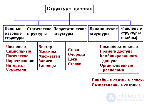
Fig. 1.1. Classification of data structures
An important feature of the data structure is the nature of the ordering of its elements. By this feature, structures can be divided into LINEAR AND NONLINEAR structures.
Depending on the nature of the mutual arrangement of elements in memory, linear structures can be divided into structures with a sequential distribution of elements in memory (vectors, rows, arrays, stacks, queues) and structures with a LINK-LINKED distribution of elements in memory (simply connected, doubly linked lists). An example of nonlinear structures is multiply connected lists, trees, and graphs.
In programming languages, the concept of "data structures" is closely related to the concept of "data types". Any data, i.e. constants, variables, values of functions or expressions are characterized by their types.
Information for each type uniquely identifies:
Subsequent chapters of this manual deal with data structures and their corresponding data types. When describing basic (simple) types and when constructing complex types, we focused mainly on the PASCAL language. This language has been used in all illustrative examples. PASCAL was created by N. Wirth specifically to illustrate data structures and algorithms and is traditionally used for these purposes. A reader familiar with any other general-purpose procedural programming language (C, FORTRAN, ALGOL, PL / 1, etc.) will easily find similar tools in a language he knows.
Four general operations can be performed on any data structures: create, destroy, select (access), update.
The creation operation is to allocate memory for the data structure. Memory can be allocated during program execution or at compile time. In a number of languages (for example, in C) for structured data constructed by the programmer, the creation operation also includes setting the initial values of the parameters of the structure being created.
For example, in PL / 1, the DECLARE N FIXED DECIMAL statement will result in the allocation of address space for the variable N. In FORTRAN (Integer I), in PASCAL (I: integer), in C (int I), as a result of the type declaration, memory will be allocated for the corresponding variables. For data structures declared in the program, the memory is automatically allocated by means of programming systems either at the compilation stage or when the procedural block is activated, in which the corresponding variables are declared. The programmer can also allocate memory for data structures himself, using the procedures / functions for allocating / releasing memory in the programming system. In object-oriented programming languages, when developing a new object, the creation and destruction procedures must be defined for it.
The main thing is that, regardless of the programming language used, the data structures in the program do not appear "out of nothing", but are explicitly or implicitly declared by structure creation statements. As a result, all instances of structures in the program are allocated memory for their placement.
The operation to destroy data structures is the opposite in its operation of the creation operation. Some languages, such as BASIC, FORTRAN, do not allow the programmer to destroy the created data structures. In PL / 1, C, PASCAL languages, the data structures that are inside the block are destroyed during the execution of the program upon exiting this block. The kill operation helps efficiently use memory.
The select operation is used by programmers to access data within the structure itself. The form of the access operation depends on the type of data structure being accessed. The access method is one of the most important properties of structures, especially since this property is directly related to the choice of a specific data structure.
The update operation allows you to change the data values in the data structure. An example of an update operation is an assignment operation, or, a more complex form is the transfer of parameters.
The above four operations are required for all structures and data types. In addition to these general operations, for each data structure, specific operations that work only with data of this type (this structure) can be defined. Specific operations are considered when considering each specific data structure.
Most authors of publications devoted to the structures and organization of data place the main emphasis on the fact that knowledge of the data structure makes it possible to organize their storage and processing in the most efficient way - from the point of view of minimizing the costs of both memory and processor time. Another, but perhaps more important, advantage that is provided by the structural approach to data is the ability to structure a complex software product. Modern industrially produced software packages are extremely complex products, the volume of which amounts to thousands and millions of lines of code, and the complexity of development is hundreds of man-years. Naturally, it is impossible to develop such a software product “all at once”; it must be presented in the form of some kind of structure - components and links between them.Proper product structuring makes it possible at each development stage to focus the developer’s attention on one observable part of the product or to entrust the implementation of its different parts to different performers.
When structuring large software products, it is possible to apply an approach based on the structuring of algorithms known as “top-down” design or “top-down programming”, or an approach based on data structuring and known as “upstream” design or “bottom-up programming”.
In the first case, the actions that the program must perform are structured primarily. The large and complex task facing the projected software product is presented in the form of several subtasks of a smaller size. Thus, the top-level module, which is responsible for solving the entire task as a whole, is quite simple and provides only a sequence of calls to modules that implement subtasks. At the first design stage, subtask modules are executed in the form of “stubs”. Then each subtask, in turn, is decomposed by the same rules. The process of crushing into subtasks continues until, at the next level of decomposition, a subtask is obtained, the implementation of which will be quite observable. In the limiting case, decomposition can be brought tothat the subtasks of the lowest level can be solved by elementary tools (for example, one operator of the selected programming language).
Another approach to structuring is based on data. A programmer who wants his program to have a real use in a certain application area should not forget that programming is data processing. In programs, you can invent arbitrarily sophisticated and sophisticated algorithms, but the real software product always has a customer. The customer has input data, and he wants to get output data for him, and what means it provides is not interested in him. Thus, the task of any software product is to convert input data to output. Programming tools provide a set of basic (simple, primitive) data types and operations on them. Integrating the base types, the programmer creates more complex data types and defines new operations on complex types. It is possible here to draw an analogy with the construction work: the basic types are the "bricks" from which complex types are created - the "building blocks". The “building blocks” compositions obtained in the first step are used as a base set for the next step, the result of which will be even more complex data constructions and even more powerful operations on them, etc. Ideally, the last step of the composition gives the data types corresponding to the input and output data of the task, and operations on these types implement in full the task of the project.
Programmers who have a superficial understanding of structured programming often oppose a top-down design to an upstream, adhering to one of their chosen approaches. The implementation of any real project is always carried out by counter paths, and with constant correction of the structures of the algorithms based on the results of the development of data structures and vice versa.
Encapsulation is another extremely productive method for data structuring. Its meaning is that the constructed data type - "building block" - is designed in such a way that its internal structure becomes inaccessible to the programmer - a user of this type. A programmer who uses this type of data in his program (in a higher-level module) can deal with data of this type only through calls to procedures defined for this type. A new data type is presented to it as a “black box” for which the inputs and outputs are known, but the content is unknown and inaccessible.
Encapsulation is extremely useful both as a means of overcoming complexity and as a means of protecting against errors. The first goal is achieved due to the fact that the complexity of the internal structure of a new data type and algorithms for performing operations on it is excluded from the programmer’s view of the user. The second goal is achieved by the fact that user access is limited to only known correct input points, therefore, the probability of errors is reduced.
Modern block-type programming languages (PASCAL, C) have sufficiently developed possibilities for building programs with a modular structure and controlling the access of modules to data and procedures. Extensions of languages with additional features for constructing types and encapsulating them make the language object-oriented. Designed and fully private data types are objects, and the procedures that work with their internal structure are the methods for working with objects. At the same time, the very concept of programming changes to a large extent. The programmer who handles objects indicates in the program what to do with the object, and not HOW it should be done.
Database technology has evolved in parallel with the technology of programming languages and is not always consistent with it. Partly this, and partly the objective differences in the nature of the problems solved by database management systems (DBMS) and programming systems, caused some terminological and conceptual differences in the approach to data in these two areas. The key concept in a DBMS is the concept of a data model, basically identical to the concept of a logical data structure. Note that the physical data structure in the database is not considered at all. But the DBMS themselves are software packages that map the physical structure into a logical one (into a data model). To implement these packages, one or another programming system is used; DBMS developers, therefore, deal with data structures in terms of programming systems. For the user, the internal structure of the DBMS and the physical structure of the data are completely transparent; it deals only with the data model and with other logical level concepts.

Comments
To leave a comment
Structures and data processing algorithms.
Terms: Structures and data processing algorithms.