Lecture
Static structures belong to the category of non-primitive structures, which, in fact, are a structured set of primitive, basic structures. For example, a vector can be represented by an ordered set of numbers. Since by definition, static structures are distinguished by a lack of variability, memory is allocated for them automatically — usually at the compilation stage or during execution — at the time of activation of the program block in which they are described. A number of programming languages (PL / 1, ALGOL-60) allow static structures to be placed in memory at the execution stage by the explicit request of the programmer, but even in this case the amount of allocated memory remains unchanged until the structure is destroyed. Memory allocation at the compilation stage is such a convenient feature of static structures that in a number of tasks programmers even use them to represent objects that have variability. For example, when the size of an array is unknown in advance, the maximum possible size is reserved for it.
Each data structure is characterized by its logical and physical representations. Very often speaking about a particular data structure, we mean its logical representation. The physical representation usually does not correspond to the logical one, and in addition, it can vary significantly in different software systems. Often, the physical structure is associated with a descriptor, or header, which contains general information about the physical structure. The descriptor is necessary, for example, in the case when the boundary values of the indices of array elements are unknown at the compilation stage, and, therefore, memory allocation for the array can be performed only at the program execution stage (as in the PL / 1 language, ALGOL-60). The descriptor is stored as the physical structure itself, in memory and consists of the fields, the nature, the number and size of which depend on the structure that it describes and on the accepted methods of its processing. In some cases, the descriptor is absolutely necessary, since the execution of the operation of accessing the structure requires the knowledge of some of its parameters, and these parameters are stored in the descriptor. Other parameters stored in the descriptor are not absolutely necessary, but using them allows you to shorten the access time or to ensure control of the correctness of access to the structure. The data structure descriptor supported by programming languages is “invisible” to the programmer; it is created by the compiler and the compiler, forming object codes for accessing the structure, includes commands referring to the descriptor to these codes.
Static structures in programming languages are associated with structured types. Structured types in programming languages are those integration tools that allow you to build data structures of arbitrarily great complexity. These types include: arrays, records (in some languages - structures) and sets (this type is not implemented in all languages).
Logical structure
A vector (one-dimensional array) is a data structure with a fixed number of elements of the same type of type. Each element of the vector has a unique number within the given vector. The call to the vector element is performed by the vector name and the number of the required element.
Machine view. Addressing elements of structures.
Vector elements are placed in memory in consecutively located memory cells. Under the vector element, the number of memory bytes is allocated, which is determined by the basic type of the element of this vector. The required number of bytes of memory to store one element of a vector is called a slot. The size of the memory for storing the vector is determined by multiplying the slot length by the number of elements.
In programming languages, a vector is represented by a one-dimensional array with the syntax of the description of the form (PASCAL):
: array [n..k] of ;
where n is the number of the first element, k is the number of the last element. The memory representation of the vector will be as shown in Fig. 3.1.
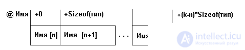
Fig. 3.1. Vector representation in memory
where @ is the name of the vector address or, equivalently, the address of the first element of the vector,
Sizeof (type) is the size of the slot (the number of bytes of memory for recording one element of the vector), (kn) * Sizeof (type) is the relative address of the element with the number k, or, equivalently, the offset of the element with the number k.
  For example:
      var m1: array [-2..2] of real;
the representation of this vector in memory will be as in fig. 3.2.

Fig. 3.2. The representation of the vector m1 in memory
In languages where memory is allocated before program execution at the compilation stage (C, PASCAL, FORTRAN), when describing the type of vector, the boundary values of the indices must be determined. In languages where memory can be dynamically allocated (ALGOL, PL / 1), index values can be set during program execution.
The number of bytes of a continuous memory area occupied simultaneously by a vector is determined by the formula:
ByteSise = (k - n + 1) * Sizeof (type)
Appeal to the i-th element of the vector is performed at the address of the vector plus the offset to this element. The offset of the i-th element of the vector is determined by the formula:
  ByteNumer = (i- n) * Sizeof (type),
 and its address: @ ByteNumber = @ name + ByteNumber.
where @name is the address of the first element of the vector.
  For example:
      var МAS: array [5..10] of word.
The basic type of a vector element - Word requires 2 bytes, so two bytes are allocated for each element of the vector. Then table 3.1 of the displacements of the vector elements relative to @Mas looks like this:
| Offset (bytes) | + 0 | + 2 | + 4 | + 6 | + 8 | + 10 |
| Field id | MAS [5] | MAS [6] | MAS [7] | MAS [8] | MAS [9] | MAS [10] |
Table 3.1
This vector will occupy in memory: (10-5 + 1) * 2 = 12 bytes.
The offset to the element of the vector with the number 8: (8-5) * 2 = 6
The address of the element with the number 8: @ MAS + 6.
When accessing a vector, the vector name and the element number of the vector are specified. Thus, the address of the i-th element can be calculated as:
@ Name [i] = @ Name + i * Sizeof (type) - n * Sizeof (type) (3.1)
This calculation cannot be performed at compile time, as the value of the variable i is still unknown at this time. Therefore, the calculation of the address of the element must be made at the stage of program execution at each reference to an element of the vector. But for this, at the execution stage, first, the parameters of formula (3.1) must be known: @ The name is Sizeof (type), n, and secondly, two multiplications and two operations must be performed at each conversion. Transforming formula (3.1) into formula (3.2),
  @ Name [i] = A0 + i * Sizeof (type) - (3.2)
          A0 = @ Name - n * Sizeof (type) -
reduce the number of stored parameters to two, and the number of operations to one multiplication and one addition, since the value of A0 can be calculated at the compilation stage and saved together with Sizeof (type) in the vector descriptor. Usually, the boundary values of the indices are saved in the vector descriptor. Each time a vector element is accessed, the specified value is compared with the boundary values and the program crashes if the specified index is out of acceptable limits.
Thus, the information contained in the vector descriptor, allows, firstly, to reduce the access time, and secondly, provides verification of the correctness of the treatment. But for these advantages, you have to pay, firstly, with speed, since references to the descriptor are commands, and secondly, with memory both for the placement of the descriptor itself and the commands that work with it.
Is it possible to do without a vector descriptor?
In the C language, for example, a vector descriptor is missing, more precisely, it is not stored at the execution stage. Indexing arrays in C necessarily starts from zero. The compiler replaces each call to an array element with a sequence of commands that implements a special case of formula (3.1) with n = 0:
@ Name [i] = @ Name + i * Sizeof (type)
Programmers who are used to working on C, often instead of expressing the form: Name [i] use an expression of the form: * (Name + i).
But firstly, the restriction in the choice of the initial index in itself can be an inconvenience for the programmer, and secondly, the absence of the boundary values of the indices makes it impossible to control the output outside the array. C programmers are well aware that it is these errors that often cause the C program to "hang" when debugging it.
An array is a data structure characterized by:
Another definition: an array is a vector, each element of which is a vector.
The syntax for describing an array is in the form:
: Array [n1..k1] [n2..k2] .. [nn..kn] of .
For the case of a two-dimensional array:
  Mas2D: Array [n1..k1] [n2..k2] of , or
       Mas2D: Array [n1..k1, n2..k2] of
A visually two-dimensional array can be represented as a table of (k1-n1 + 1) rows and (k2-n2 + 1) columns.
The physical structure is the placement of the elements of the array in the computer memory. For the case of a two-dimensional array consisting of (k1-n1 + 1) rows and (k2-n2 + 1) columns, the physical structure is shown in fig. 3.3.

Fig. 3.3. The physical structure of a two-dimensional array of (k1-n1 + 1) rows and (k2-n2 + 1) columns
Multidimensional arrays are stored in a continuous memory area. The size of the slot is determined by the basic type of the array element. The number of array elements and the size of the slot determine the size of the memory for storing the array. The principle of the distribution of array elements in memory is determined by the programming language. So in FORTRAN elements are distributed in columns - so that the left indices change faster, in PASCAL - in rows - the indices change in the direction from right to left.
The number of bytes of memory occupied by a two-dimensional array is determined by the formula:
ByteSize = (k1-n1 + 1) * (k2-n2 + 1) * SizeOf (Type)
The array address is the address of the first byte of the initial component of the array. The offset to the element of the array Mas [i1, i2] is determined by the formula:
  ByteNumber = [(i1-n1) * (k2-n2 + 1) + (i2-n2)] * SizeOf (Type)
 His address is @ByteNumber = @mas + ByteNumber.
      For example:
      var Mas: Array [3..5] [7..8] of Word;
The basic type of the Word element requires two bytes of memory, then table 3.2 of the displacements of the array elements relative to @Mas will be as follows:
| Offset (bytes) | Field id | Offset (bytes) | Field id |
| + 0 | Mas [3.7] | + 2 | Mas [3,8] |
| + 4 | Mas [4.7] | +6 | Mas [4.8] |
| + 8 | Mas [5,7] | + 10 | Mas [5.8] |
Table 3.2
This array will occupy in memory: (5-3 + 1) * (8-7 + 1) * 2 = 12 bytes; and the address of the element Mas [4,8]:
@Mas + ((4-3) * (8-7 + 1) + (8-7) * 2 = @ Mas + 6
The most important physical level operation on an array is access to a given element. As soon as access to the element is realized, it can be performed on any operation that makes sense for the type of data to which the element corresponds. The transformation of a logical structure into a physical one is called a linearization process, during which the multidimensional logical structure of an array is transformed into a one-dimensional physical structure.
In accordance with formulas (3.3), (3.4) and by analogy with the vector (3.1), (3.2) for a two-dimensional array with the limits of change of indices:
[B (1) .. E (1)] [B (2) .. E (2)] located in the memory in rows, the address of the element with the indices [I (1), I (2)] can be calculated as :
  Addr [I (1), I (2)] = Addr [B (1), B (2)] +
  {[I (1) -B (1)] * [E (2) -B (2) +1] + [I (2) -B (2)]} * SizeOf (Type) (3.5)
      Summarizing (3.5) for an array of arbitrary dimension:
            Mas [B (1) .. E (2)] [B (2) .. E (2)] ... [B (n) .. E (n)]
 we will receive:
      Addr [I (1), I (2), ..., I (n)] = Addr [B (1), B (2), ... B (n)] -
                 nn (3.6)
 - Sizeof (Type) * SUM [B (m) * D (m)] + Sizeof (Type) * SUM [I (m) * D (m)]
                m = 1 m = 1
where Dm depends on the way the array is placed. When placing in rows:
D (m) = [E (m + 1) -B (m + 1) +1] * D (m + 1), where m = n-1, ..., 1 and D (n) = 1
when placed in columns:
D (m) = [E (m-1) -B (m-1) +1] * D (m-1), where m = 2, ..., n and D (1) = 1
When calculating the address of an element, the most difficult is to calculate the third component of formula (3.6), since the first two do not depend on indices and can be calculated in advance. To speed up the calculations, the factors D (m) can also be calculated in advance and stored in the array descriptor. The array descriptor thus contains:
One of the definitions of the array says that it is a vector, each element of which is a vector. Some programming languages allow you to select one or more dimensions from a multidimensional array and treat them as an array of smaller dimensionality.
For example, if a two-dimensional array is declared in a PL / 1 program:
DECLARE A (10,10) BINARY FIXED;
This expression: A [*, I] - will refer to a one-dimensional array consisting of the elements: A (1, I), A (2, I), ..., A (10, I).
The joker symbol "*" means that all elements of the array are selected by the dimension corresponding to the index given by the joker. Using the joker also allows you to specify group operations on all the elements of the array or on its selected dimension,
for example: A (*, I) = A (*, I) + 1
The logical level operations on arrays should include such as sorting an array, searching for an item by key. The most common search and sorting algorithms will be discussed later in this chapter.
It can be seen from the above formulas that the calculation of the address of the element of a multidimensional array can take a lot of time, since it requires addition and multiplication operations, the number of which is proportional to the dimension of the array. The multiplication operation can be eliminated by using the following method.
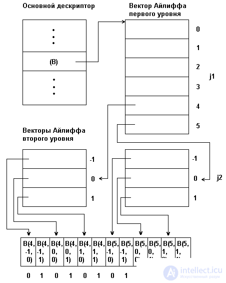
Fig. 3.4. Array representation using Eiliff vectors
For an array of any dimensionality, a set of descriptors is formed: the main one and several levels of auxiliary descriptors, called Ailiff vectors. Each Ailiff vector of a defined level contains a pointer to the zero components of the Ailiff vectors of the next lower level, and the Ailiff vectors of the lowest level contain pointers of groups of elements of the displayed array. The main array descriptor stores the first-level Ailiff vector pointer. With such an organization, an arbitrary element B (j1, j2, ..., jn) of a multidimensional array can be accessed by traversing the chain from the main descriptor through the corresponding components of the Ailiff vectors.
In fig. 3.4 shows the physical structure of the three-dimensional array in [4..5, -1..1.0 ..1], presented by the method of Ailiff. This figure shows that, by increasing the speed of access to the elements of an array, the Ailiff method leads at the same time to an increase in the total amount of memory required to represent the array. This is the main drawback of the representation of arrays with the aid of the Eiliff vectors.
In practice, there are arrays that, due to certain reasons, can be written into memory not completely, but partially. This is especially true for arrays so large in size that it may not be enough to store them in full memory. These arrays include symmetric and sparse arrays.
Symmetric arrays.
A two-dimensional array in which the number of rows equals the number of columns is called a square matrix. A square matrix in which the elements located symmetrically relative to the main diagonal are pairwise equal to each other is called symmetric. If a matrix of order n is symmetric, then in its physical structure it is enough to display not n ^ 2, but only n * (n + 1) / 2 eI elements. In other words, only the top (including the diagonal) triangle of a square logical structure must be represented in memory. Access to a triangular array is organized in such a way that it is possible to refer to any element of the initial logical structure, including elements whose values, although not represented in memory, can be determined based on the values of elements symmetric to them.
In practice, procedures are developed for working with a symmetric matrix for:
a) convert the indices of the matrix in the index vector,
b) forming a vector and writing elements of the upper triangle of elements of the original matrix into it,
c) obtaining the value of the matrix element from its packed representation. With this approach, the appeal to the elements of the original matrix is performed indirectly, through the specified functions.
The appendix contains an example of a program for working with a symmetric matrix.
Sparse arrays.
A sparse array is an array, most of the elements of which are equal to each other, so only a small number of values other than the main (background) values of the remaining elements are sufficient to be kept in memory.
There are two types of sparse arrays:
In the case of working with sparse arrays, the issues of their placement in the memory are implemented at the logical level, taking into account their type.
Arrays with a mathematical description of the location of non-background elements.
To this type of arrays are arrays, in which the locations of elements with values different from the background, can be mathematically described, that is, there is a pattern in their location.
Элементы, значения которых являются фоновыми, называют нулевыми; элементы, значения которых отличны от фонового, - ненулевыми. Но нужно помнить, что фоновое значение не всегда равно нулю.
Ненулевые значения хранятся, как правило, в одномерном массиве, а связь между местоположением в исходном, разреженном, массиве и в новом, одномерном, описывается математически с помощью формулы, преобразующей индексы массива в индексы вектора.
На практике для работы с разреженным массивом разрабатываются функции:
При таком подходе обращение к элементам исходного массива выполняется с помощью указанных функций. Например, пусть имеется двумерная разреженная матрица, в которой все ненулевые элементы расположены в шахматном порядке, начиная со второго элемента. Для такой матрицы формула вычисления индекса элемента в линейном представлении будет следующей : L=((y-1)*XM+x)/2), где L - индекс в линейном представлении; x, y - соответственно строка и столбец в двумерном представлении; XM - количество элементов в строке исходной матрицы.
В программном примере 3.1 приведен модуль, обеспечивающий работу с такой матрицей (предполагается, что размер матрицы XM заранее известен).
 {===== Программный пример 3.1 =====} Unit ComprMatr;
  Interface
  Function PutTab(y,x,value : integer) : boolean;
  Function GetTab(x,y: integer) : integer;
  Implementation
  Const XM=...;
  Var arrp: array [1..XM * XM div 2] of integer;
  Function NewIndex (y, x: integer): integer;
     var i: integer;
     begin NewIndex: = ((y-1) * XM + x (div 2);  end;
  Function PutTab (y, x, value: integer): boolean;
      begin
        if NOT ((x mod 2 <> 0) and (y mod 2 <> 0)) or
           NOT ((x mod 2 = 0) and (y mod 2 = 0)) then begin
              arrp [NewIndex (y, x)]: = value; PutTab: = true; end
                                              else PutTab: = false;
      end;
  Function GetTab (x, y: integer): integer;
      begin
        if ((x mod 2 <> 0) and (y mod 2 <> 0)) or
           ((x mod 2 = 0) and (y mod 2 = 0)) then GetTab: = 0
        else GetTab: = arrp [NewIndex (y, x)];
      end;
 end.
The compressed representation of the matrix is stored in the arrp vector.
The NewIndex function recalculates the indexes using the above formula and returns the index of the element in the arrp vector.
The PutTab function stores in a compressed representation of a single element with x, y indices and a value value. Saving is performed only if the indices x, y address an element that is not obviously zero. If the save is done, the function returns true; otherwise, it returns false.
To access an element by indices of a two-dimensional matrix, the function GetTab is used, which returns the selected value by indices x, y. If the indices address the obviously zero element of the matrix, the function returns 0.
Note that the arrp array as well as the NewIndex function are not described in the module’s IMPLEMENTATION section. Access to the contents of the matrix from the outside is possible only through the input points PutTab, GetTab with the assignment of two indices.
In program example 3.2, the same problem is solved in a slightly different way: for the matrix, a descriptor is created — the desc array, which is filled when the matrix is initialized so that the i-th element of the desc array contains the index of the first element of the i-th row of the matrix in its linear representation. InitTab initialization procedure is included in the number of input points of the module and must be called before working with the matrix. But access to each element of the matrix (the NewIndex function) is simplified and faster: by the row number y, the index of the beginning of the row is immediately selected from the descriptor and the offset of the element from the column x is added to it. The procedures PutTab and GetTab are the same as in Example 3.1, therefore they are not listed here.
 {===== Software Example 3.2 =====}
 Unit ComprMatr;
  Interface
  Function PutTab (y, x, value: integer): boolean;
  Function GetTab (x, y: integer): integer;
  Procedure InitTab;
  Implementation
  Const XM = ...;
  Var arrp: array [1..XM * XM div 2] of integer;
      desc: array [1..XM] of integer;
  Procedure InitTab;
  var i: integer;
    begin
      desc [1]: = 0; for i: = 1 to XM do desc [i]: = desc [i-1] + XM;
    end;
  Function NewIndex (y, x: integer): integer;
  var i: integer;
  begin NewIndex: = desc [y] + x div 2;  end;
 end.
Sparse arrays with randomly arranged elements.
This type of arrays includes arrays whose locations of elements with values different from the background cannot be mathematically described, that is, there is no pattern in their location.
 E 0 0 6 0 9 0 0 E
Ё 2 0 0 7 8 0 4 Ё
Ё10 0 0 0 0 0 0 Ё
Ё 0 0 12 0 0 0 0 Ё
Ё 0 0 0 3 0 0 5 Ё
Let there be a matrix A of dimension 5 * 7, in which out of 35 elements only 10 are non-zero.
Представление разреженным матриц методом последовательного размещения.
Один из основных способов хранения подобных разреженных матриц заключается в запоминании ненулевых элементов в одномерном массиве и идентификации каждого элемента массива индексами строки и столбца, как это показано на рис. 3.5 а).
Доступ к элементу массива A с индексами i и j выполняется выборкой индекса i из вектора ROW, индекса j из вектора COLUM и значения элемента из вектора A. Слева указан индекс k векторов наибольшеее значение, которого определяется количеством нефоновых элементов. Отметим, что элементы массива обязательно запоминаются в порядке возрастания номеров строк.
Более эффективное представление, с точки зрения требований к памяти и времени доступа к строкам матрицы, показано на рис.3.5.б). Вектор ROW уменьшнен, количество его элементов соответствует числу строк исходного массива A, содержащих нефоновые элементы. Этот вектор получен из вектора ROW рис. 3.5.а) так, что его i-й элемент является индексом k для первого нефонового элемента i-ой строки.
Представление матрицы А, данное на рис. 3.5 сокращает требования к объему памяти более чем в 2 раза. Для больших матриц экономия памяти очень важна. Способ последовательного распределения имеет также то преимущество, что операции над матрицами могут быть выполнены быстрее, чем это возможно при представлении в виде последовательного двумерного массива, особенно если размер матрицы велик.
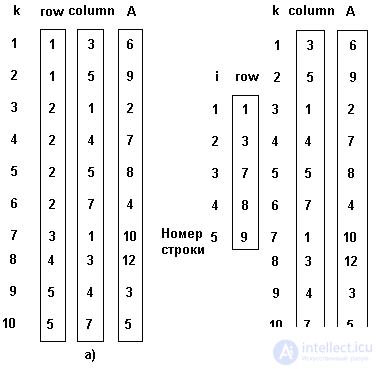
Fig. 3.5. Последовательное представление разреженных матриц.
Представление разреженных матриц методом связанных структур.
Методы последовательного размещения для представления разреженных матриц обычно позволяют быстрее выполнять операции над матрицами и более эффективно использовать память, чем методы со связанными структурами. Однако последовательное представление матриц имеет определенные недостатки. Так включение и исключение новых элементов матрицы вызывает необходимость перемещения большого числа других элементов. Если включение новых элементов и их исключение осуществляется часто, то должен быть выбран описываемый ниже ме- тод связанных структур.
Метод связанных структур, однако, переводит представляемую структуру данных в другой раздел классификации. При том, что логическая структура данных остается статической, физическая структура становится динамической.
Для представления разреженных матриц требуется базовая структура вершины (рис.3.6), называемая MATRIX_ELEMENT ("элемент матрицы"). Поля V, R и С каждой из этих вершин содержат соответственно значение, индексы строки и столбца элемента матрицы. Поля LEFT и UP являются указателями на следующий элемент для строки и столбца в циклическом списке, содержащем элементы матрицы. Поле LEFT указывает на вершину со следующим наименьшим номером строки.
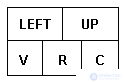
Рис.3.6. Формат вершины для представления разреженных матриц
In fig. 3.7 приведена многосвязная структура, в которой используются вершины такого типа для представления матрицы А, описанной ранее в данном пункте. Циклический список представляет все строки и столбцы. Список столбца может содержать общие вершины с одним списком строки или более. Для того, чтобы обеспечить использование более эффективных алгоритмов включения и исключения элементов, все списки строк и столбцов имеют головные вершины. Головная вершина каждого списка строки содержит нуль в поле С; аналогично каждая головная вершина в списке столбца имеет нуль в поле R. Строка или столбец, содержащие только нулевые элементы, представлены головными вершинами, у которых поле LEFT или UP указывает само на себя.

Fig. 3.7. Многосвязная структура для представления матрицы A
Может показаться странным, что указатели в этой многосвязной структуре направлены вверх и влево, вследствие чего при сканировании циклического списка элементы матрицы встречаются в порядке убывания номеров строк и столбцов. Такой метод представления используется для упрощения включения новых вершин в структуру. Предполагается, что новые вершины, которые должны быть добавлены к матрице, обычно располагаются в порядке убывания индексов строк и индексов столбцов. Если это так, то новая вершина всегда добавляется после головной и не требуется никакого просмотра списка.
Логическая структура.
Множество - такая структура, которая представляет собой набор неповторяющихся данных одного и того же типа. Множество может принимать все значения базового типа. Базовый тип не должен превышать 256 возможных значений. Поэтому базовым типом множества могут быть byte, char и производные от них типы.
Физическая структура.
Множество в памяти хранится как массив битов, в котором каждый бит указывает является ли элемент принадлежащим объявленному множеству или нет. So максимальное число элементов множества 256, а данные типа множество могут занимать не более 32-ух байт.
Число байтов, выделяемых для данных типа множество, вычисляется по формуле: ByteSize = (max div 8)-(min div 8) + 1, где max и min - верхняя и нижняя границы базового типа данного множества.
Номер байта для конкретного элемента Е вычисляется по формуле:
ByteNumber = (E div 8) - (min div 8),
bit number inside this byte by the formula:
BitNumber = E mod 8
 {===== Software Example 3.3 =====}
     const max = 255; min = 0; E = 13;
     var S: set of byte;
          ByteSize, ByteNumb, BitNumb: byte;
      begin
        S: = []; {null set}
        S: = S + [E]; {write number to set}
        ByteSize: = (max div 8) - (min div 8) +1;
        Bytenumb: = (E div 8) - (min div 8);
        BitNumb: = E mod 8;
        writeln (bytesize); {on screen 32}
        writeln (bytenumb); {on screen 1}
        writeln (bitnumb); {on screen 5}
      end.
The standard numeric type, which can be the base for the formation of a set is the byte type.
The set is stored in memory as shown in Table 3.3.
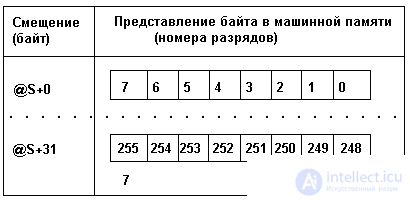
Table 3.3
where @S is the address of this type set.
The field bit is set to 1 if the element is in the set, and to 0 if it is not.
For example, S: set of byte; S: = [15,19];
    The contents of the memory will be as follows:
   @ S + 0 - 00000000 @ S + 2 - 00001000
   @ S + 1 - 10,000,000.  .  .  .  .  .
                       @ S + 31 - 00000000
Character sets are stored in memory as well as numeric sets. The only difference is that not numbers are stored, but ASCII character codes.
For example, S: set of char; S: = ['A', 'C'];
In this case, the representation of the set S in memory is as follows:
 @ S + 0 - 00000000.  .  .  .  .  .
    .  .  .  .  .  . @ S + 31 - 00000000
   @ S + 8 - 00001010
A set whose base type is an enumerated type is also stored as a set whose base type is a byte type. However, it takes up space in memory, which depends on the number of elements in the enumerated type.
  Example:
       Type
         Video = (MDA, CGA, HGC, EGA, EGAm, VGA, VGAm, SVGA, PGA, XGA);
       Var
         S: set of Video;
The memory will occupy:
ByteSize = (9 div 8) - (0 div 8) + 1 = 2 bytes.
In this case, the memory for the variable S will be allocated as shown in Fig. 3.8.
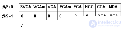
Fig. 3.8. Memory allocation for a variable of type set of video
If you execute the operator S: = [CGA, SVGA], the contents of the memory will be:
             @ S + 0 - 10000010
             @ S + 1 - 00000000
A set whose base type is an interval type is also stored as a set whose base type is a byte type. However, it takes up space in the memory, which depends on the number of elements included in the declared interval.
  For example,
       type S = 10..17;
       var I: set of S;
Это не значит, что первый элемент будет начинаться с 10-того или 0-ого бита, как может показаться на первый взгляд. Как видно из формулы вычисления смещения внутри байта 10 mod 8 = 2, смещение первого элемента множества I начнЯтся со второго бита. И, хотя множество этого интервала свободно могло поместиться в один байт, оно займЯт (17 div 8)-(10 div 8)+1 = 2 байта.
В памяти это множество имеет представление как на рис. 3.9.
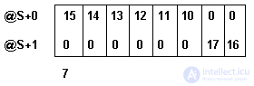
Fig. 3.9. Представление переменной типа set of S
Для конструирования множеств интервальный тип самый экономичный, т.к. занимает память в зависимости от заданных границ.
 Например, Type S = 510..520;
               Var I : S;
               begin I:=[512];  end.
     Представление в памяти переменной I будет:
     @i+0 - 00000000 @i+1 - 00000001
Let S1, S2, S3: set of byte. Over these sets the following specific operations are defined:
A record is a finite ordered set of fields characterized by a different data type. Records are an extremely convenient tool for representing program models of real objects of the domain, for, as a rule, each such object has a set of properties characterized by data of various types.
An example of a record is a collection of information about a student.
The object "student" has the properties:
  Example: var
           rec: record
               num: byte;  {student's personal number}
               name: string [20];  { FULL NAME.  }
          fac, group: string [7];  {faculty, group}
     math, comp, lang: byte;  {math scores, cal.  }
               end;  {technology, in.  language}
In memory, this structure can be represented in one of two types:
a) in the form of a sequence of fields occupying a continuous area of memory (Fig. 3.10). With such an organization, it is enough to have one pointer to the beginning of the region and an offset from the beginning. This saves memory, but is a waste of time calculating the addresses of record fields.
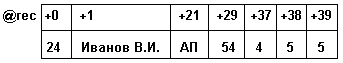
Fig. 3.10. Memory representation of a record variable as a sequence of fields
b) in the form of a linked list with pointers to the field values of the record. With such an organization, there is a quick access to the elements, but a very uneconomical consumption of memory for storage. The structure of storage in memory of a linked list with pointers to the elements is shown in Fig. 3.11.
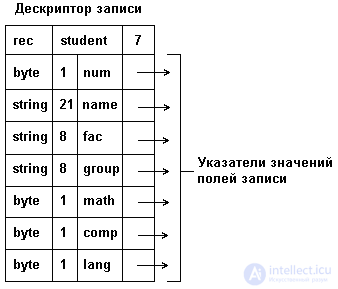
Fig. 3.11. Memory representation of a record type as a linked list.
Note: to save the amount of memory allocated for a record, the values of some of its fields are stored in the descriptor itself, instead of pointers, then the corresponding attributes should be written in the descriptor.
In accordance with the general approach of the C language, the record descriptor (in this language, records are called structures) is not saved until the program is executed. The fields of the structure are simply located in adjacent memory slots, the calls to individual fields are replaced with their addresses at the compilation stage.
The record field can in turn be an integrated data structure - a vector, an array, or another record. In some programming languages (COBOL, PL / 1), the description of nested records indicates the level of nesting, in others (PASCAL, C), the level of nesting is determined automatically.
The record field may be another record, but by no means the same. This is primarily due to the fact that the compiler must allocate memory for the recording. Suppose a record of the form is described:
  type rec = record
        f1: integer;
        f2: char [2];
        f3: rec;  end;
How will the compiler allocate memory for such a record? For the f1 field, 2 bytes will be allocated, for the f2 field - 2 bytes, and the f3 field will be a record, which in turn consists of f1 (2 bytes), f2 (2 bytes) and f3, which ... etc. Not without reason, the C compiler, upon encountering such a description, produces a message about insufficient memory.
However, the field of a record may well be a pointer to another such record: the size of the memory occupied by the pointer is known and there are no problems with memory allocation. This technique is widely used in programming to establish links between similar records (see Chapter 5).
The most important operation for recording is the operation of accessing the selected field of the record - the operation of qualification. In almost all programming languages, the designation of this operation has the form:
.
So, for the record described in the beginning of p.3.5.1, the constructions: stud1.num and stud1.math will provide references to the num and math fields, respectively.
Over the selected recording field, any operations that are valid for the type of this field are possible.
Most programming languages support some operations that work with a record as a whole, and not with its individual fields. These are the operations of assigning one record to the value of another one-type record and comparing two one-type records for equality / inequality. In the same cases when such operations are not explicitly supported by the language (C language), they can be performed on separate fields of records or the records can be copied and compared as unstructured memory areas.
In a number of applications, a programmer may encounter groups of objects whose sets of properties overlap only partially. Processing of such objects is performed using the same algorithms if the general properties of the objects are processed, or according to different ones - if specific properties are processed. It is possible to describe all groups uniformly, including in the description all sets of properties for all groups, but such a description would be uneconomical from the point of view of consumable memory and inconvenient from a logical point of view. If we describe each group with our own structure, we lose the ability to process common properties according to uniform algorithms.
For tasks of this kind, advanced programming languages (C, PASCAL) provide a programmer with a record with options. Record with options consists of two parts. The first part describes the fields common to all groups of objects modeled by the record. Among these fields there is usually a field whose value allows identifying the group to which the given object belongs and, therefore, which of the variants of the second part of the record should be used in processing. The second part of the record contains descriptions of disjoint properties — for each subset of such properties — a separate description. A programming language may require that the names of property fields do not repeat in different versions (PASCAL), or require the naming of each variant (C). In the first case, the identification of a field located in the variant part of the record when accessing it is no different from the case of a simple record:
.
In the second case, the identification is a bit more complicated:
. .
Consider the use of records with options for example. Suppose you want to place on the screen of a video terminal simple geometric shapes - circles, rectangles, triangles. For the "database", which will describe the state of the screen, it is convenient to represent all the figures in the same type of records. For any shape, its description should include the coordinates of some reference point (center, upper right corner, one of the vertices) and a color code. Other parameters of construction will be different for different shapes. So for the circle - the radius; for a rectangle - the lengths of non-parallel sides; for a triangle - the coordinates of two other vertices.
Writing with options for such a task in PASCAL language looks like:
  type figure = record
       fig_type: char;  {type of figure}
       x0, y0: word;  {coordinates of reference point}
       color: byte;  { Colour }
       case fig_t: char of
         'C': (radius: word);  {radius of circle}
         'R': (len1, len2: word);  {length of the sides of the rectangle}
         'T': (x1, y1, x2, y2: word);  {coordinates of two vertices}
       end;
and in C, like:
  typedef struct
   {char fig_type;  / * shape type * /
     unsigned int x0, y0;  / * coordinates of the reference point * /
     unsigned char color;  /* Colour */
     union
     {struct
      {unsigned int radius;  / * radius of the circle * /
      } cyrcle;
     struct
      {unsigned int len1, len2;  / * length of the sides of the rectangle * /
      } rectangle;
     struct
      {unsigned int x1, y1, x2, y2;  / * coordinates of two vertices * /
      } triangle;
     } fig_t;
   } figure;
And if the program defines a variable fig1 of the figure type, in which the description of the circle is stored, then the reference to the radius of this circle in the PASCAL language will look like: fig1.radius, and in C: fig1.circle.radius
The field named fig_type is entered to represent the identifier of the shape type, which, for example, can be encoded with the characters: "C" is a circle or "R" is a rectangle, or "T" is a triangle.
Memory allocation for recording with options is shown in Figure 3.12.
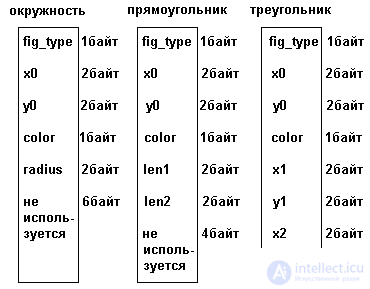
Fig.3.12. Memory allocation for recording with options
As can be seen from the figure, under the entry with options, in any case, the amount of memory sufficient to accommodate the largest option is allocated. If the allocated memory is used for a smaller variant, a part of it remains unused. The total part of the record for all variants is placed in such a way that the offsets of all fields relative to the start of the record are the same for all variants. Obviously, this is most easily achieved by placing common fields at the beginning of a record, but this is not strictly necessary. The variant part can also be “wedged in” between the fields of the common part. Since in any case the variant part has a fixed (maximum) size, the displacements of the fields of the common part will also remain fixed.
When it came to records, it was noted that record fields could be integrated data structures - vectors, arrays, and other records. Similarly, elements of vectors and arrays can also be integrated structures. One such complex structure is a table. From a physical point of view, a table is a vector whose elements are records. A characteristic logical feature of the tables, which determined their consideration in a separate section, is that access to table elements is not done by number (index), but by key - by the value of one of the object properties described by the table element entry. A key is a property that identifies a given entry in a set of similar entries. As a rule, the key is the requirement of uniqueness in this table. The key may be included in the record and be one of its fields, but it may not be included in the record, but calculated by the position of the record. A table can have one or more keys. For example, when integrating into the table of students' records (the description of the record is given in Section 3.5.1), the sample can be made according to the student's personal number or by last name.
The main operation when working with tables is a record access operation by key. It is implemented by the search procedure. Since the search can be significantly more efficient in tables sorted by key values, quite often it is necessary to perform sorting operations on tables. These operations are discussed in the following sections of this chapter.
Sometimes there are tables with fixed and variable record length. It is obvious that the tables combining records of completely identical types will have fixed record lengths. The need for a variable length may arise in tasks similar to those considered for variant records. As a rule, tables for such tasks are made up of records with variants, i.e. reduced to a fixed (maximum) record length. Much less often there are tables with really variable length of record. Although in such tables the memory is saved, but the possibilities of working with such tables are limited, since it is impossible to determine its address by the record number. Tables with records of variable length are processed only sequentially - in ascending order of record numbers. Access to an element of such a table is usually done in two steps. At the first step, the permanent part of the record is selected, which contains — explicitly or implicitly — the length of the record. In the second step, the variable part of the record is selected in accordance with its length. Adding to the address of the current record its length, get the address of the next record.
So a table with records of variable length can, for example, be considered in some problems programmed in machine codes. Each machine command - record, consists of one or several bytes. The first byte is always the operation code, the number and format of the remaining bytes is determined by the type of command. The processor selects a byte at the address specified by the program counter, and determines the type of command. According to the type of command, the processor determines its length and selects the rest of its bytes. The content of the program counter is increased by the length of the command.
In this and the following sections, a number of data retrieval and sorting algorithms performed on static data structures are presented, since these are typical logical level operations for such structures. However, the same operations and the same algorithms apply to data that have the logical structure of a table, but which are physically located in dynamic memory and external memory, as well as the logical tables of any physical representation, which have variability.
An objective criterion to evaluate the effectiveness of an algorithm is the so-called order of the algorithm. The order of the algorithm is the function O (N), which makes it possible to estimate the dependence of the execution time of the algorithm on the amount of data processed (N is the number of elements in the array or table). The efficiency of the algorithm is higher, the shorter its execution time depends on the amount of data. From the point of view of order, most algorithms are reduced to three main types:
The efficiency of power-law algorithms is usually considered poor, linear - satisfactory, and logarithmic - good.
Analytical determination of the order of the algorithm, although often difficult, is possible in most cases. The question arises: why then do we need such a variety of algorithms, for example, sorting, if it is possible to determine once and for all the algorithm with the best analytical performance indicator and leave the “right to life” solely behind it? The answer is simple: in real-world problems there are limitations determined by both the logic of the problem and the properties of a specific computing environment that can help or hinder the programmer and that can significantly affect the efficiency of this particular implementation of the algorithm. Therefore, the choice of an algorithm is always left to the programmer.
In the following, all the descriptions of the algorithms are given to work with a table consisting of the records R [1], R [2], ..., R [N] with the keys K [1], K [2], ..., K [N]. In all cases, N is the number of table elements. Software examples to reduce their size work with arrays of integers. Such an array can be considered as a degenerate case of a table, each record of which consists of a single field, which is also a key. In all program examples, the
продолжение следует...
Часть 1 3. STATIC DATA STRUCTURE
Часть 2 3.8. Операции логического уровня над статическими структурами. Sorting - 3.
Часть 3 3.8.3. Sort by distribution. - 3. STATIC DATA STRUCTURE

Comments
To leave a comment
Structures and data processing algorithms.
Terms: Structures and data processing algorithms.