4. Recursive data structures

Consider recursive algorithms and recursive data structures.

Recursion is a process, the flow of which is associated with appeal to oneself (to the same process).

An example of a recursive data structure is a data structure whose elements are the same data structures (Fig. 4.1).

4.1 Trees

Tree is a non-linear bound data structure
(Fig. 4.2).





The tree is characterized by the following features:

- The tree has 1 element that is not referenced by other elements. This element is called the root of the tree;

- in the tree, you can access any element by passing a finite number of links (pointers);

- each element of the tree is associated with only one previous element. Any node of the tree can be either intermediate or terminal (leaf). In fig. 4.2 intermediate elements are M1, M2, leaves - A, B, C, D, E. A characteristic feature of the terminal node is the absence of branches.

Height is the number of levels of the tree. At the tree in fig. 4.2 height is two.

The number of branches growing from a tree node is called the degree of outcome of the node (in Fig. 4.2 for M1, the degree of outcome is 2, for M2 - 3). By degree of outcome trees are classified:

1) if the maximum degree of outcome is m, then this is an m-ary tree;

2) if the degree of outcome is either 0 or m, then this is a complete m-ary tree;

3) if the maximum degree of outcome is 2, then this is a binary tree;

4) if the degree of outcome is either 0 or 2, then this is a complete binary tree.

The following terminology is also used to describe the connections between the nodes of the tree: M1 is the “father” for elements A and B. A and B are the “sons” of the node M1.

4.1.1 Representation of trees

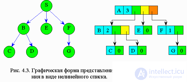
The most convenient trees to represent in the memory of a computer in the form of linked lists. The list element should contain information fields that contain the node value and the degree of outcome, as well as pointer fields, the number of which is equal to the degree of outcome (Fig. 4.3). That is, any element pointer orients this node element with the sons of this node.  

4.2 Binary trees

Binary trees are the most commonly used tree species.

According to the representation of trees in the computer memory, each element will be a record containing 4 fields. The values ​​of these fields will be respectively the key of the record, the link to the element left-down, the element to the right-down and the text of the record.

When building it is necessary to remember that the left son has a key smaller than that of the father, and the key value of the right son is greater than the key value of the father. For example, we build a binary tree of the following elements: 50, 46, 61, 48, 29, 55, 79. It has the following form:





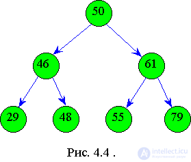
We got an ordered binary tree with the same number of levels in the left and right subtrees. This is a perfectly balanced tree, that is, a tree in which the left and right subtrees have levels that differ by no more than one.

To create a binary tree, you need to create elements of the type in memory (Fig. 4.5):





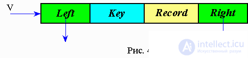
Operation V = MakeTree (Key, Rec) - creates an element (tree node) with two pointers and two fields (key and informational).


Type of MakeTree procedure:

Pseudocode p = getnode r (p) = rec k (p) = key v = p left (p) = nil right (p) = nil

Pascal New (p); p ^ .r: = rec; p ^ .k: = key; v: = p; p ^ .left: = nil; p ^ .right: = nil;

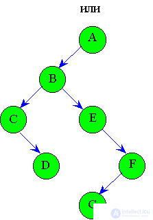
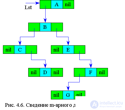
4.2.1 M-ary tree reduction to binary

Informal algorithm:


1. In any node of the tree, all branches are cut off, except the leftmost one, corresponding to the eldest sons.

2. The horizontal lines are all the sons of the same parent.

3. The eldest son in any node of the resulting structure will be the node under the given node (if any).

The sequence of actions of the algorithm is shown in Fig. 4.6.

2. Basic tree operations

1. Bypassing the tree.

2. Delete the subtree.

3. Insert a subtree.


To perform a tree walk , you must perform three procedures:

1. Processing of the root.

2. Processing of the left branch.

3. Processing of the right branch.


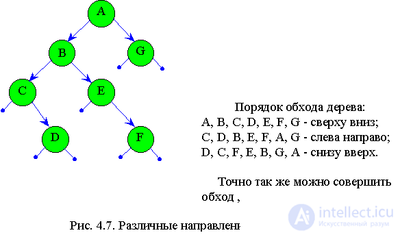
Depending on the sequence in which these three procedures are performed, there are three types of workarounds.

1. Turning from top to bottom. Procedures are performed in sequence.

1-2-3.

2. Turn left to right. Procedures are performed in sequence.

2 - 1 - 3.

3. Turning up from the bottom. Procedures are performed in sequence.

2 - 3 -1.


Depending on which entry in the node leads to the processing of the node, it turns out the implementation of one of the three types of bypass. If the processing goes after the first entry into the node, then from top to bottom, if after the second, then from left to right, if after the third, then from bottom to top (see. Fig. 4. 7).





The operation to exclude a subtree. You must specify the node to which the excluded subtree is connected and the index of this subtree. The exception of a subtree is that the connection with the excluded subtree is broken, i.e. the element pointer is set to nil, and the outcome of this node is reduced by one.

Inserting a subtree is the inverse operation of an exception. You need to know the index of the included subtree, the node to which the tree is suspended, set the pointer of this node to the root of the subtree, and the degree of outcome of this node is increased by one. In this case, it is generally necessary to renumber the sons of the node to which the subtree is suspended.

The insertion and deletion algorithm is discussed in Chapter 5.

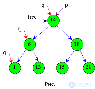
4.2.3 Algorithm for creating a binary search tree

Let the elements with the keys be set: 14, 18, 6, 21, 1, 13, 15. After executing the algorithm below, you will get the tree shown in Fig.4.6. If we go around the resulting tree from left to right, we get the ordering: 1, 6, 13, 14, 15, 18, 21.

Pseudocode read (key, rec) tree = maketree (key rec) p = tree q = tree while not eof do read (key, rec) v = maketree (key, rec) while p <> nil do q = p if key <k (p) then p = left (p) else p = right (p) endif endwhile if key <k (q) then left (p) = v else right (p) = v endif if q = tree then 'root only' endif return

Pascal read (key, rec); tree: = maketree (key rec); p: = tree; q: = tree; while not eof do begin read (key, rec); v: = maketree (key, rec); while p <> nil do begin q: = p; if key <p ^ .k then p: = p ^ .left else p: = p ^ .right; end; if key <q ^ .k then p ^ .left: = v else p ^ .right: = v; end if q = tree then writeln ('Root only'); exit

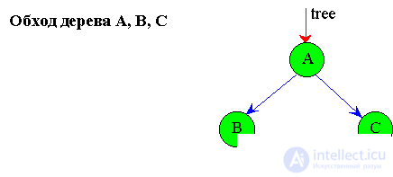
4.2.4 Passage of binary trees

Depending on the sequence of traversing subtrees, there are three types of traversing (passing) of trees (Fig.4.9):





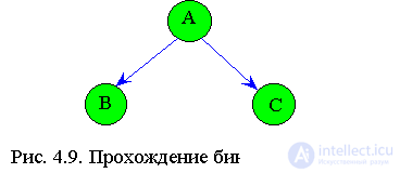
1. From top to bottom A, B, C.

2. From left to right or symmetrical passage B, A, C.

3. Bottom up B, C, A.


The second method is most often used.

Below are the recursive algorithms for passing binary trees.

subroutine pretrave (tree) 'top to bottom if tree <> nil then print info (tree) pretrave (left (tree)) pretrave (right (tree)) endif return subroutine intrave (tree) 'symmetrical if tree <> nil then intrave (left (tree)) print info (tree) intrave (right (tree)) endif return

Procedure pretrave (tree: tnode) Begin if tree <> nil then begin WriteLn (Tree ^ .Info); Pretrave (Tree ^ .left); Pretrave (Tree ^ .right); End; end; procedure intrave (tree: tnode) begin if tree <> nil then begin intrave (Tree ^ .left); writeLn (Tree ^ .info); intrave (Tree ^ .right); end; end;

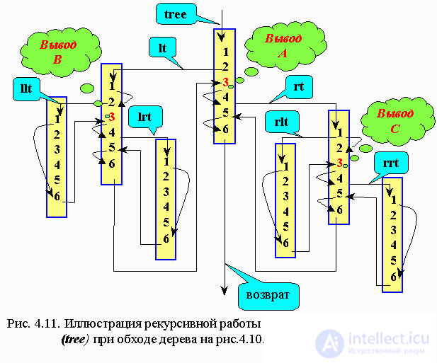
Let us explain in more detail the recursion of the tree traversal algorithm from left to right.

Number the algorithm strings.   intrave ( tree ):

1. 
   if tree <> nil
2. 
   then intrave (left (tree))
3. 
   print info (tree)
4. 
   intrave (right (tree))
5. 
   endif
6. 
   return

Denote pointers: t → tree; l → left; r → right

In the above figure. 4.11 illustrates the sequence of calling the intrave ( tree ) procedure as you traverse the nodes of the simplest tree shown in Figure. 4. 10.